Session 2 - Digitization and georeferencing of raster data

23 Jan 2022

Advanced GIS · Sciences Po Urban School

Lecturer: Raphaëlle Roffo

 

I. Session 2 Overview

Download the slides

• Some raster dataset examples
• Georeferencing: use cases
• Georeferencing: understanding the different types of transformation
• Digitization

 

II. Tutorial

Goals:

• Polygonizing a raster layer
• Georeferencing a PDF or image
• Digitizing features to create a new vector layer

 

Download the data

Create an Advanced-Session2 folder, and download the data in this folder. Add the folder to your Favourites in QGIS to have an easy access to it.

• Output from Session 1
• Satellite imagery

III. Polygonize

We ended last session with a classification of the vegetation across an area spanning across West London. Based on this output, you might now want to create a vector dataset of certain features you’re able to detect based on that index value. For instance, water bodies are clearly visible (the river Thames, reservoirs and lakes, the Lea River, etc).

One way to create a new class bases on this classification is to use the raster to vector conversion. This tool is available under the top Raster menu > Conversions > Polygonize (Raster to Vector. The tool will basically group together pixels with the same value and draw boundaries around them to create polygons (remember that our band has been reclassified to only have five possible values: 0, 1, 2, 3 or 4).

 

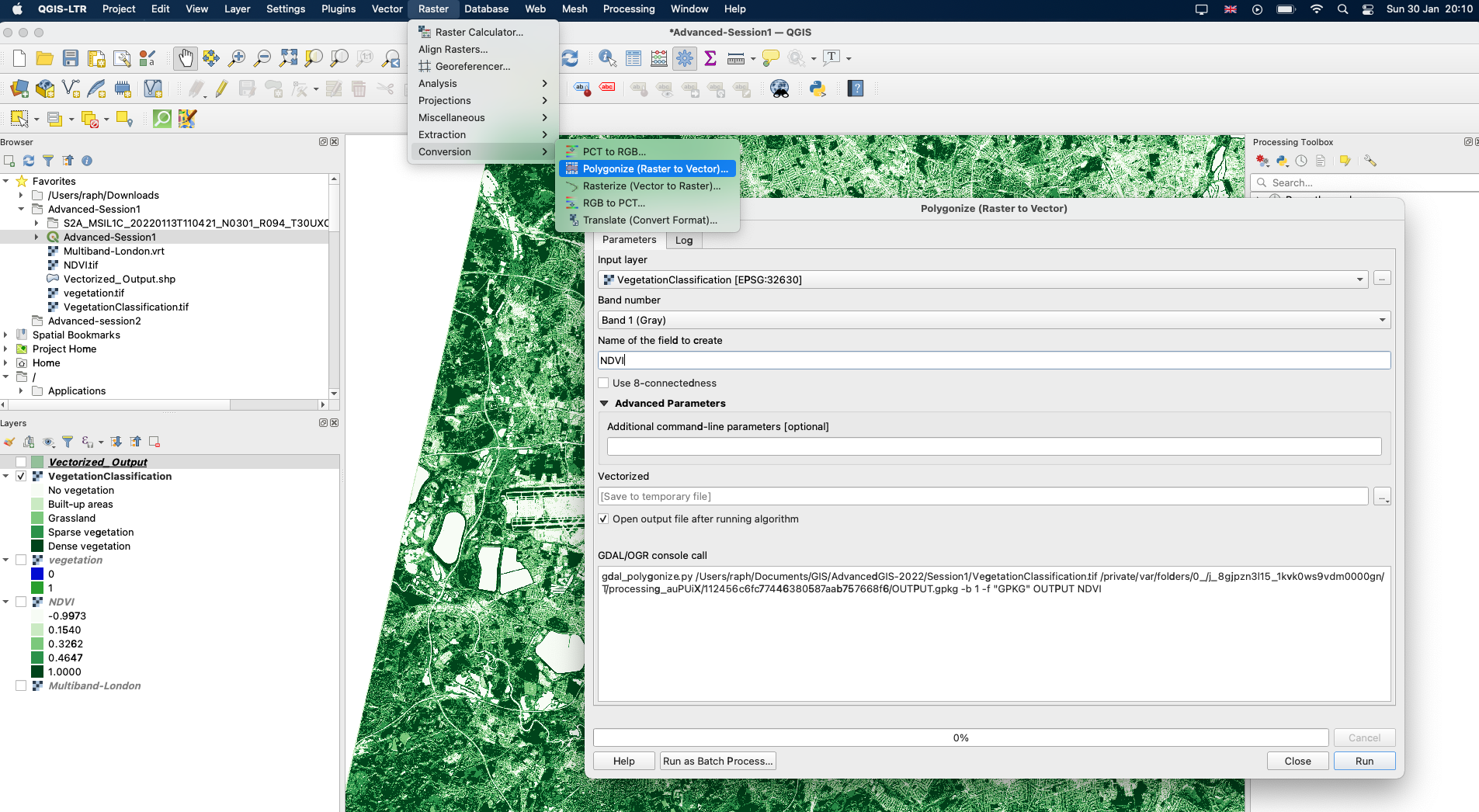
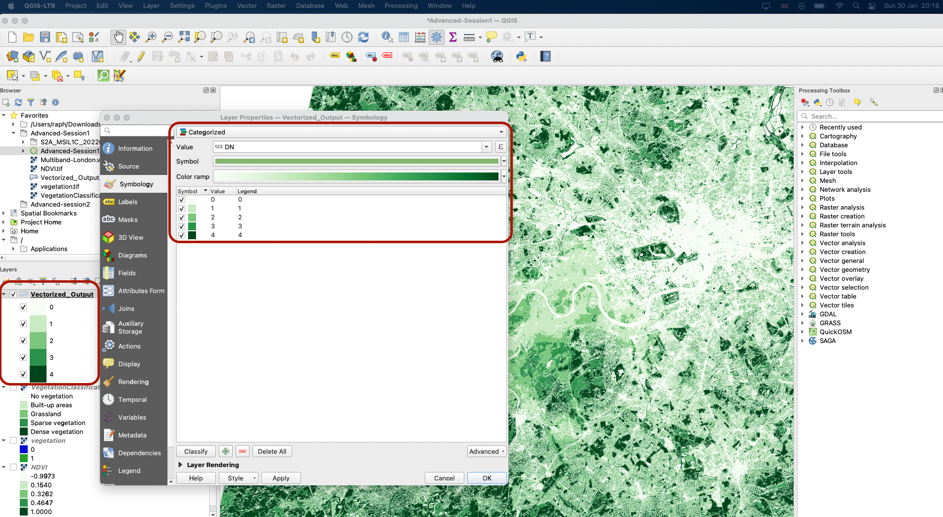
Because the tool requires quite a lot of computing power, it would take a long time to run on your computer - you do not have to do it. I have run it and saved the vector output as Vectorized_Output.shp. Turn this layer on; I’ve applied a categorical symbology and a green ramp to then display it.

 

If you zoom in and use the query tool, you will see that polygons were indeed created, but their boundaries still represent the shape of the pixels. You might also notice that in some cases the pixels are very mixed and it is difficult to see any big polygon emerge.

 

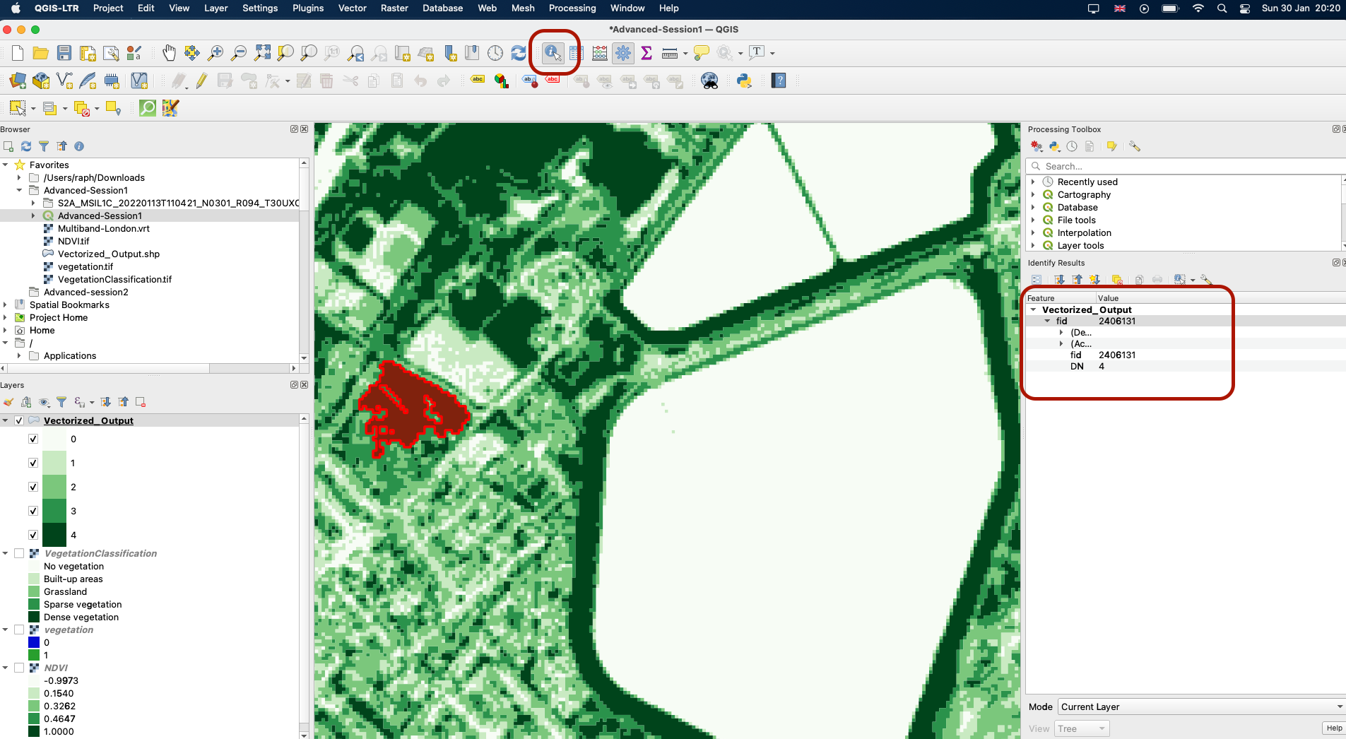
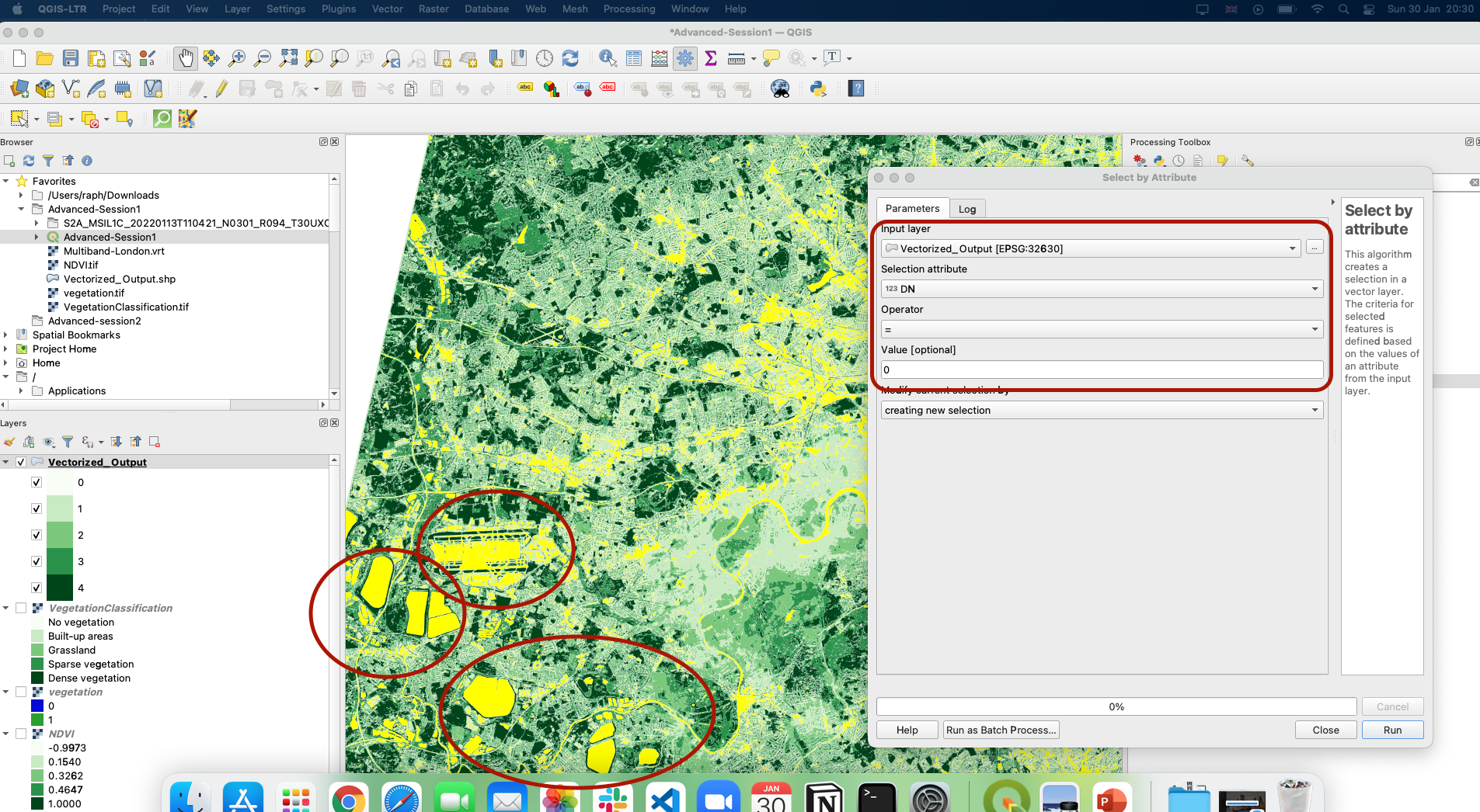
The water bodies and built-up surfaces such as Heathrow airport are however very clearly visible. We can use the Select by attribute tool to select all the polygons representing the Vegetation Index value of 0 = “No vegetation”, and see those polygons selected in yellow:

 

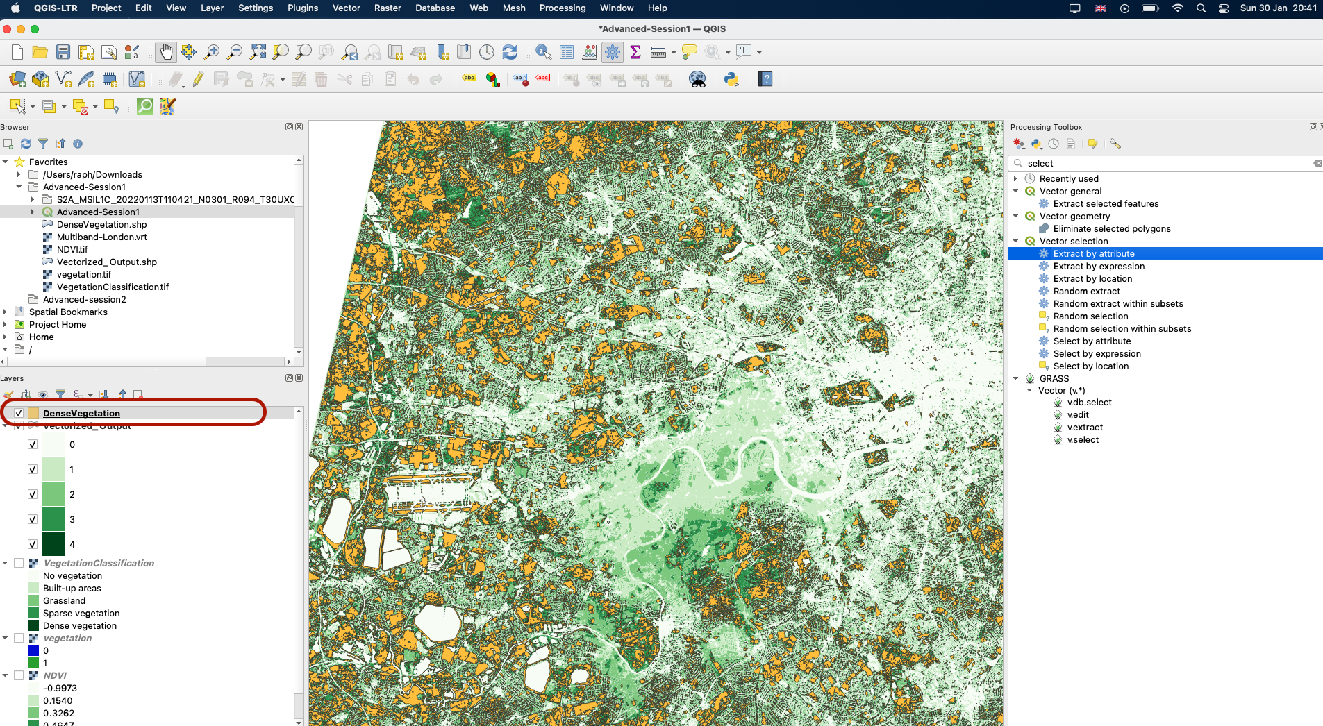
We can also use Extract by attribute to create a new layer of these polygons. For instance, let’s create a new layer with the polygons representing a Dense Vegetation (value of 4 in our VegetationClassification layer):

 

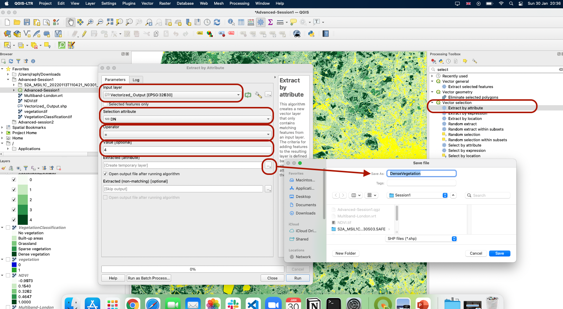
You can skip this step as it may also take some time to run on your computer. The output of this extraction is a new vector layer, which we call DenseVegetation and you may now use in other analyses (for instance, you may want to count the surface of dense vegetation in each borough and put in in perspective with socio-economic status of the population).

 

IV. Georeferencing

4.1 Overview

In some other cases, you might want to create your own vector layer. Let’s imagine that you have an image of a map or a satellite image, and you are interested in creating a new dataset with some of the pictures you are seeing. In order to digitise the features you are interested in, you will first need to georeference your image; then, you will be able to build your new dataset using the digitizing tools.

In this section, we are going to take a satellite image of London; a 1m resolution panchromatic (meaning black and white) IKONOS image from 2008 that does not have spatial references. We are going to create those spatial references, using a basemap and points that we can easily identify on both the basemap and the photo.

You can close the Session1 file and open a new empty file. Save the project as Advanced-Session2. Drag and drop the sat.tif file onto your canvas

 

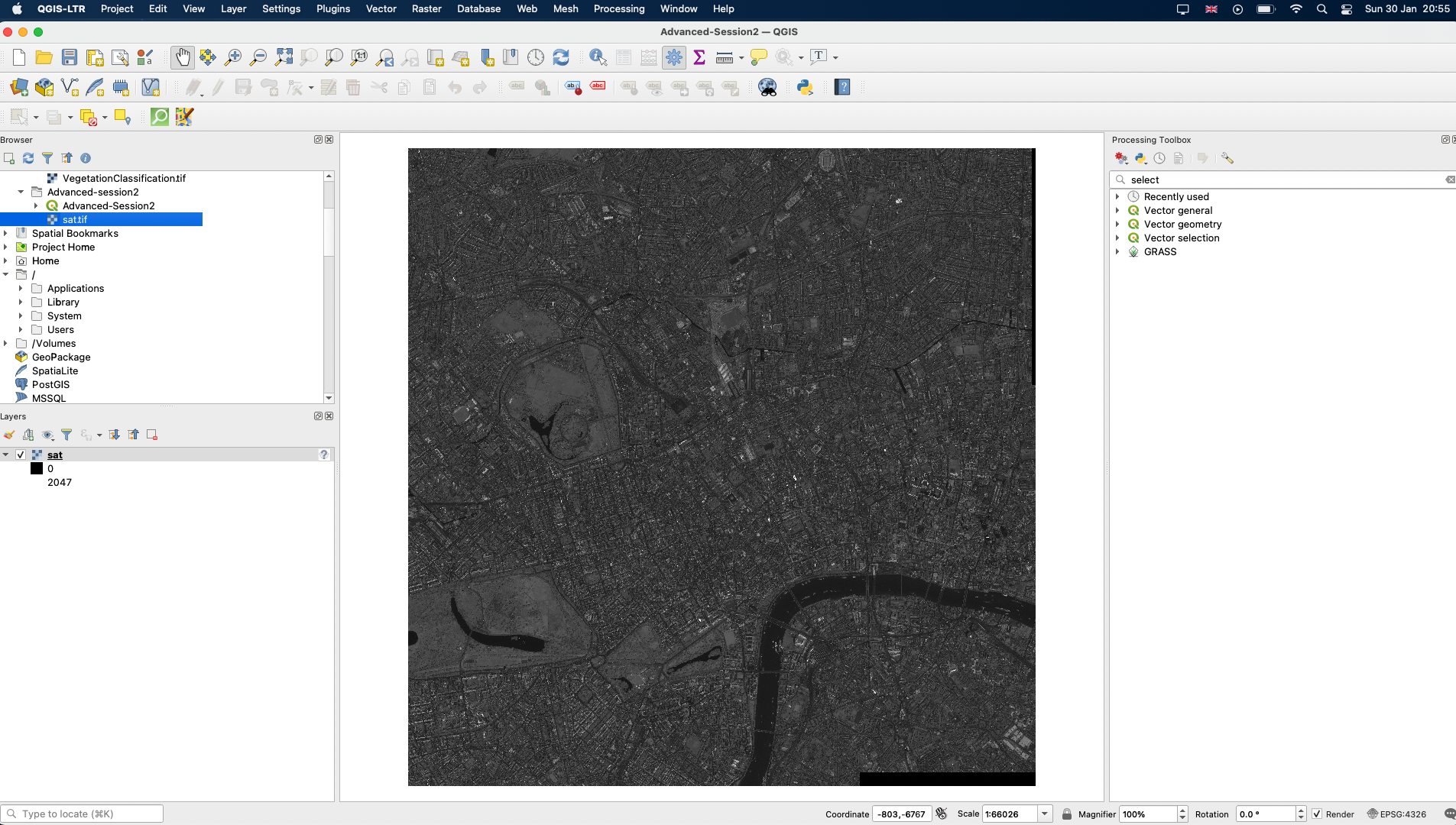
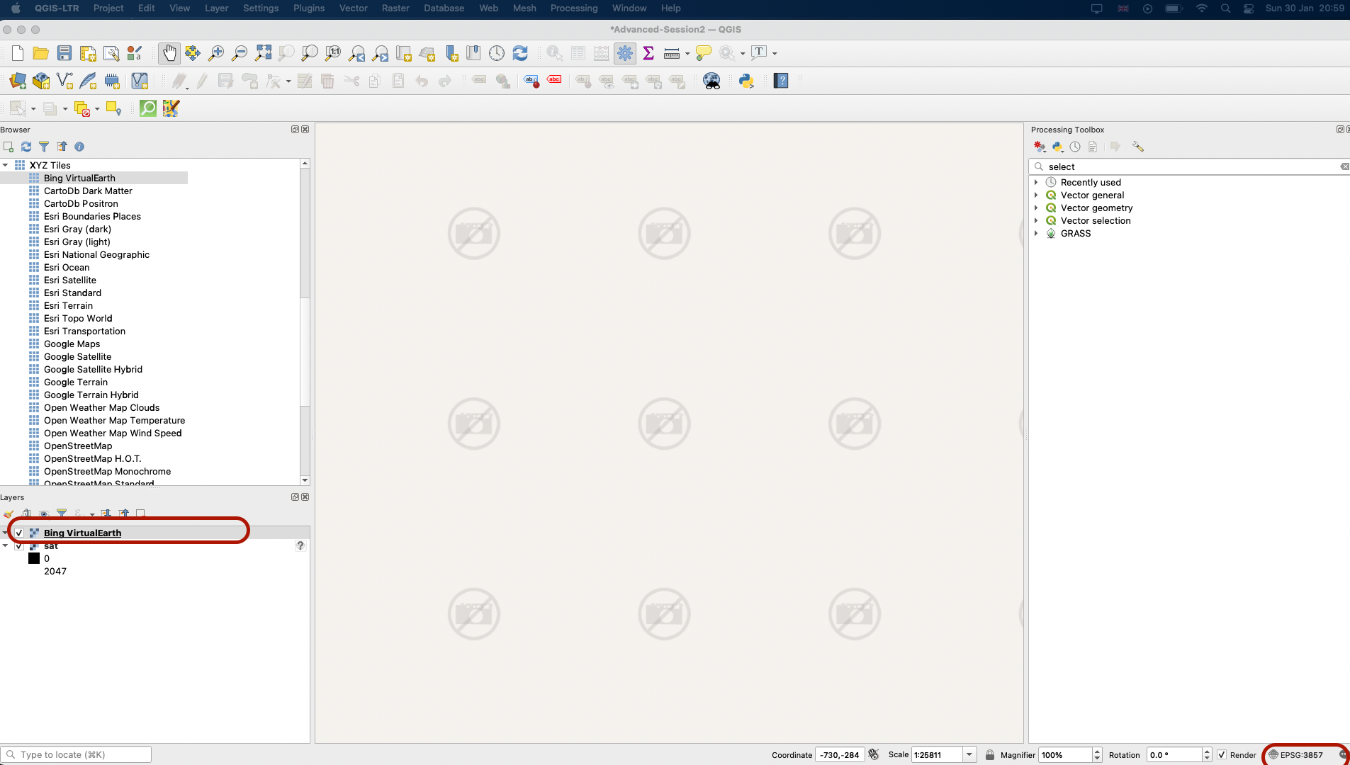
Now, this image does not actually contain any spatial reference. In your browser if you turn on one of your basemaps (preferably Bing VirtualEarth), you will see that it is absolutely not placing your image in London: yours might be different but on my computer, I get this barred camera sign. Before we go any further, check your CRS: because we are using a basemap that uses Web Mercator coordinates, make sure your project CRS is indeed set to Web Mercator: EPSG:3857

 

You can now remove the sat.tif layer from your canvas, right click your basemap layer > Zoom to layer to find your basemap again, and zoom onto London. To get there, you can also paste -5524,6704409 into your Coordinates and enter and 1:50000 into the scale.

 

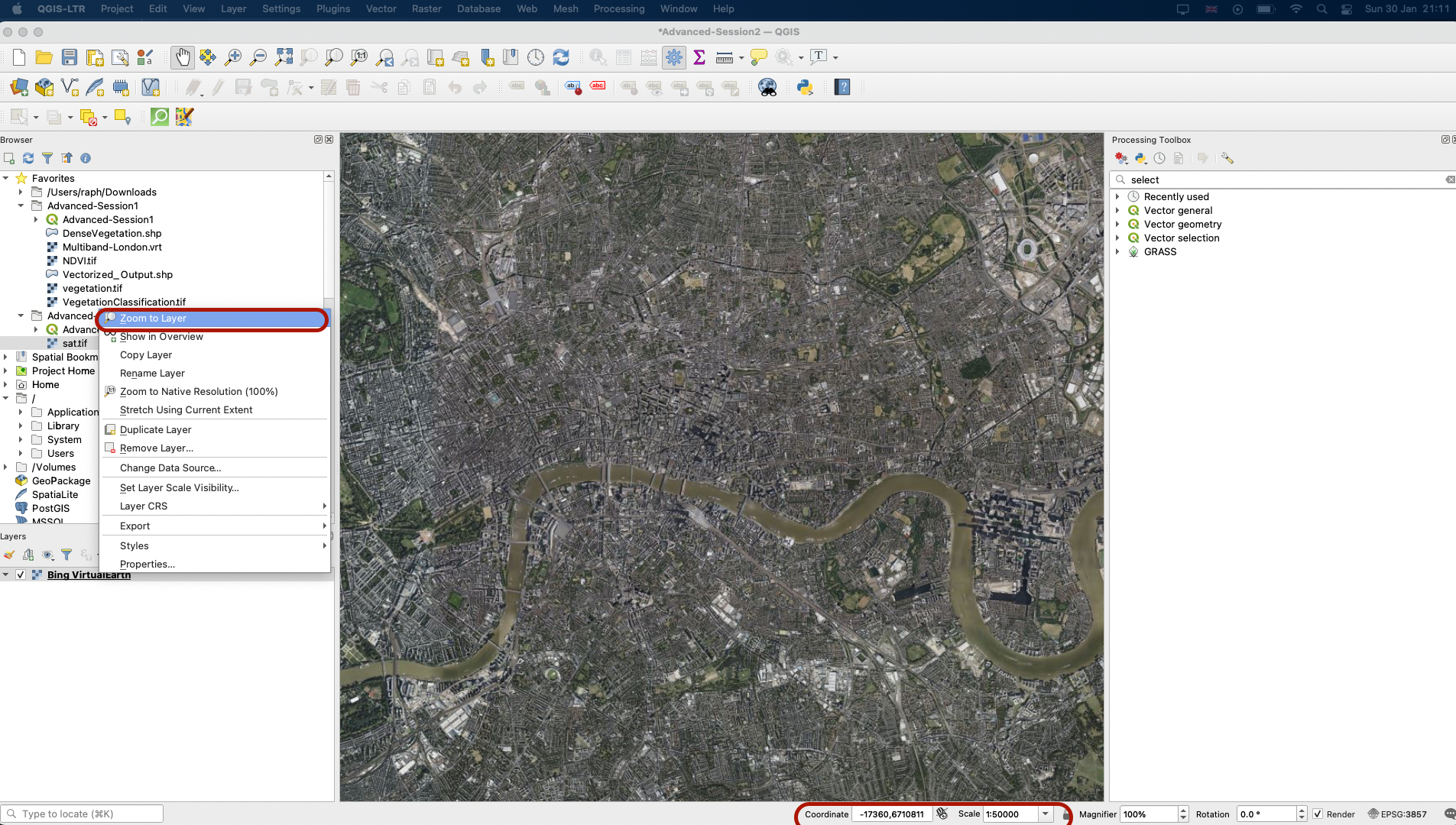
4.2 Georeferencing tool

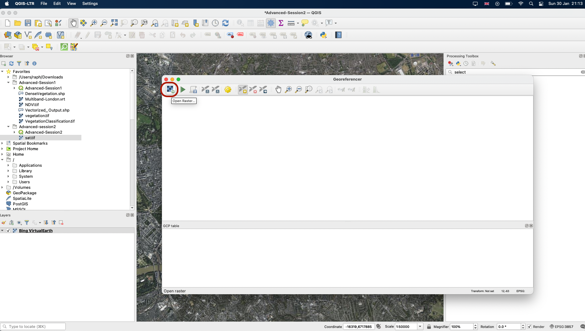
In your top Raster menu, click on Georeferencer; a white window opens. Click on the Open Raster button and select your sat.tif file.

 

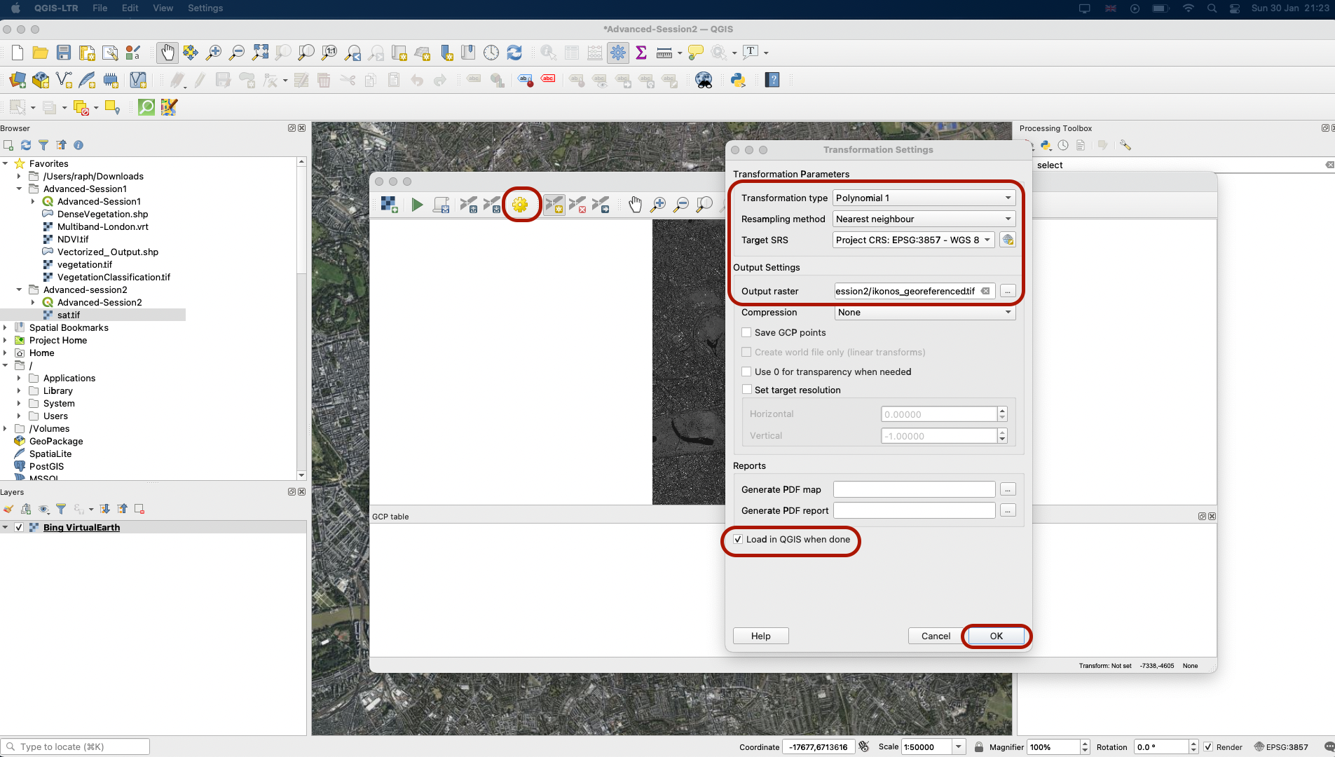
Next, click on the yelow cogwheel to open the Transformation Settings. We will be using a Polynomial 1 transformation type (= Affine). With this type of transformation, you will introduce a potential scale change, rotation angle, a shift on the x axis and the y-axis, and a change in the angles of your raster cells. In general, this transformation works well and tends to not overly distort the image. It also requires less Ground Control Points (GCP). Pick Nearest neighbour as resampling method, and EPSG:3857 as the target CRS. Youc an then click on the three dots next to Output Raster to specify a name and location for your new georeferenced image. You can save it in your Advanced-Session2 folder as ikonos_georeferenced.tif. Finally, make sure Load in QGIS when done box is ticked. Press OK.

 

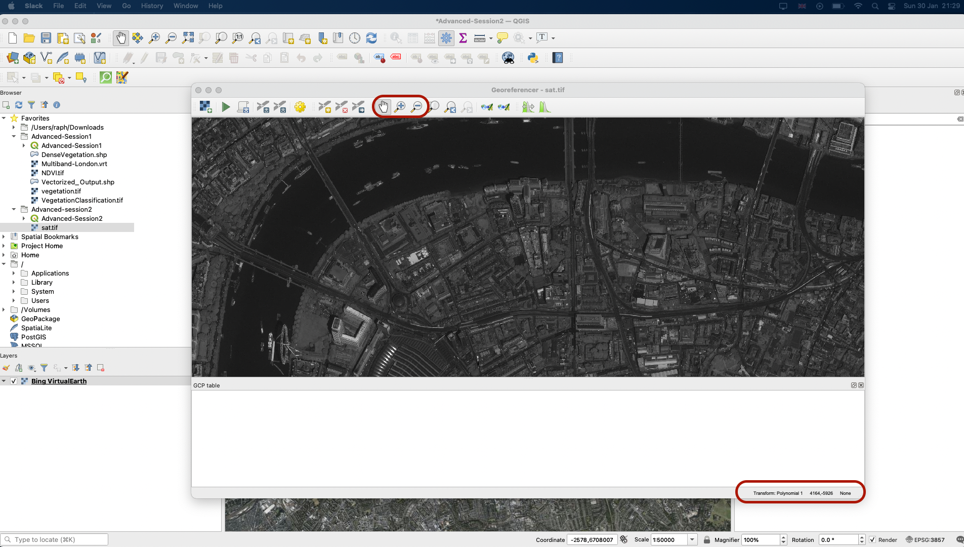
4.3 Defining Ground Control Points

Now at the bottom of your window you can see a summary of the transformation. We will be monitoring the transformation error (RMSE); for now its value is None as no Ground Control Points have been set. For now, use the white glove to pan across your image and zoom in and out with your mouse scroll. Find some notable points that you could easily spot on your basemap. For instance, the edge of bridges, a crossroads, the corner of a large building or a landmark can be easy points to match. We will aim to find 4 to 6 points, nicely distributed across the picture (this is important to reduce error).

 

Notice that there is an important difference between the image and your basemap: on your image you can see the sides of buildings at an angle, while on the Bing basemap the image has been orthorectified, meaning you see each building as if you were perfectly on top of it, and you don’t see the side of buildings and houses.

I am going to place my first point on the North pillar at the base of the London Eye. To do so, click the point you have spotted. A pop-up window asks you for the coordinates; use From map canvas and click the point location on your basemap. The (x,y) coordinates will then automatically be populated in your Georeferencer window. Press OK.

 

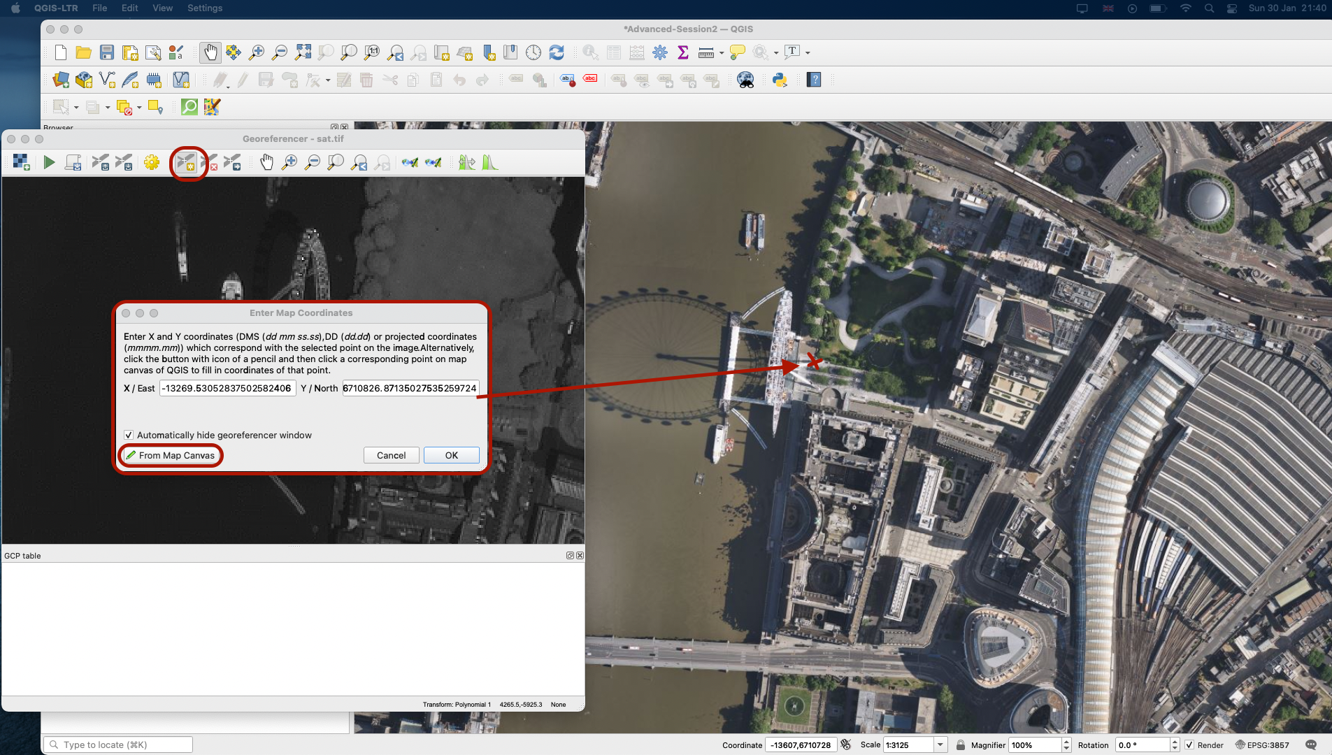
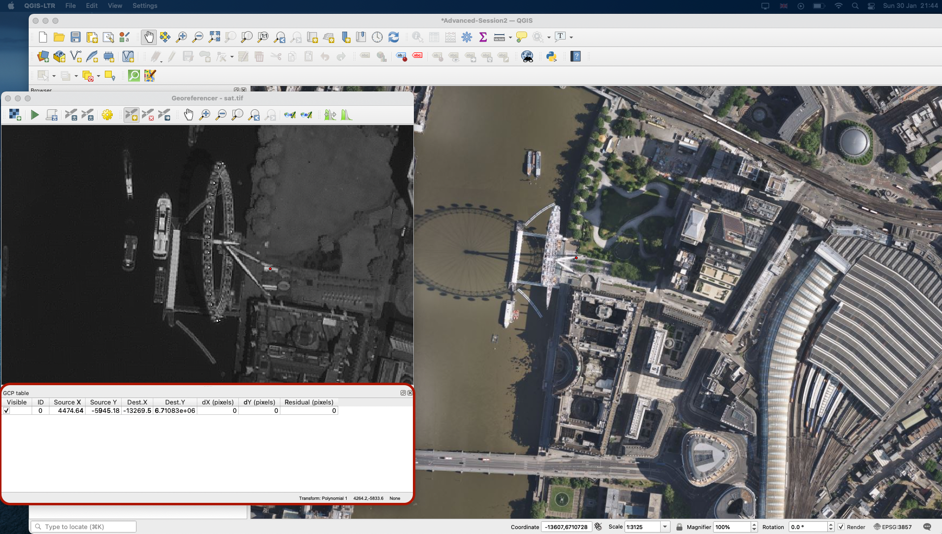
A GCP table has now appeared at the bottom of your Georeferencer, and a red point marks your first point, GCP 0, on both your image and the basemap.

 

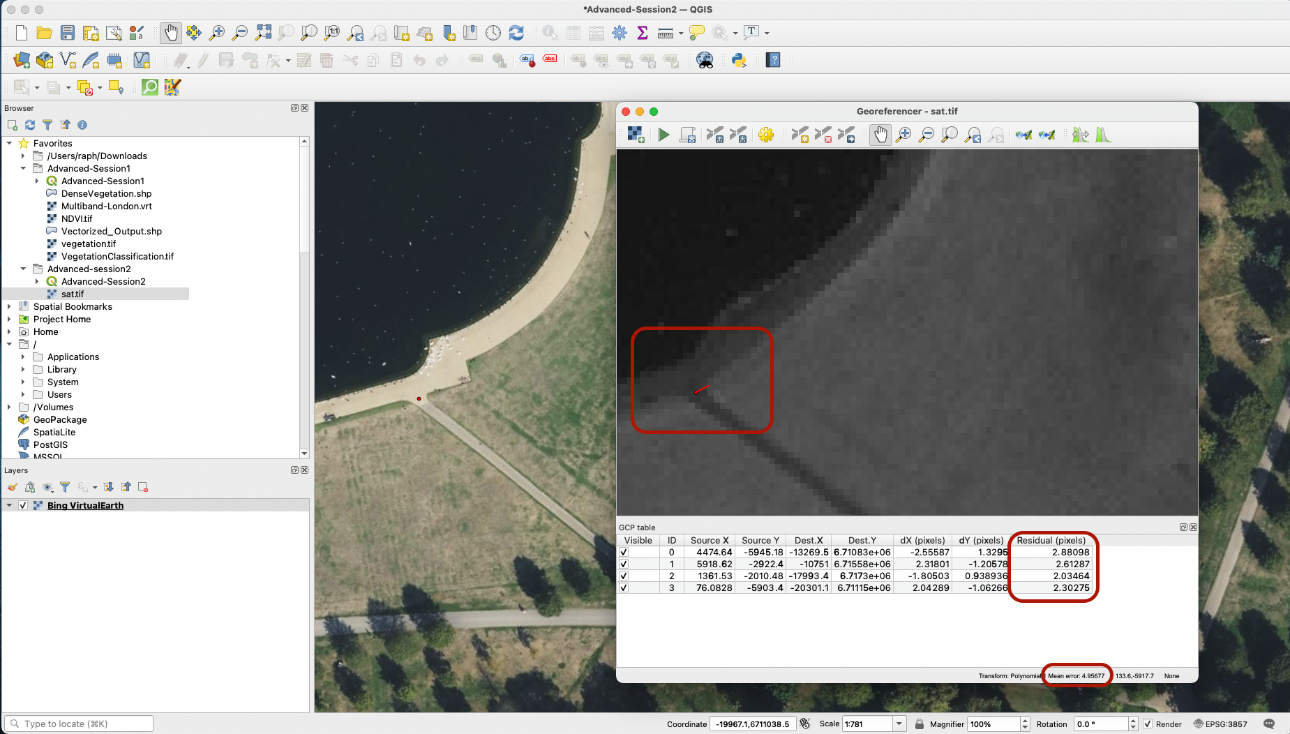
Repeat the operation a few times with points spread across your image, until you have 4 rows (0 to 3) in your table. Once you pin your 4th point, you might get a red line next to your point: This actually represents the residual error of your transformation equation. This matches the Residual value in the table, which represents how far the transformation fit value is from our expected fit value calculated with the other points. If one point is very much off and has a considerably higher residual value than other points, you might want to check again this point, and maybe delete it or modify it using the delete/edit GCP buttons.

Notice the Mean error value at the bottom: this represents the overall error of your transformation equation. You can try and reduce the error by adding a couple more points.

 

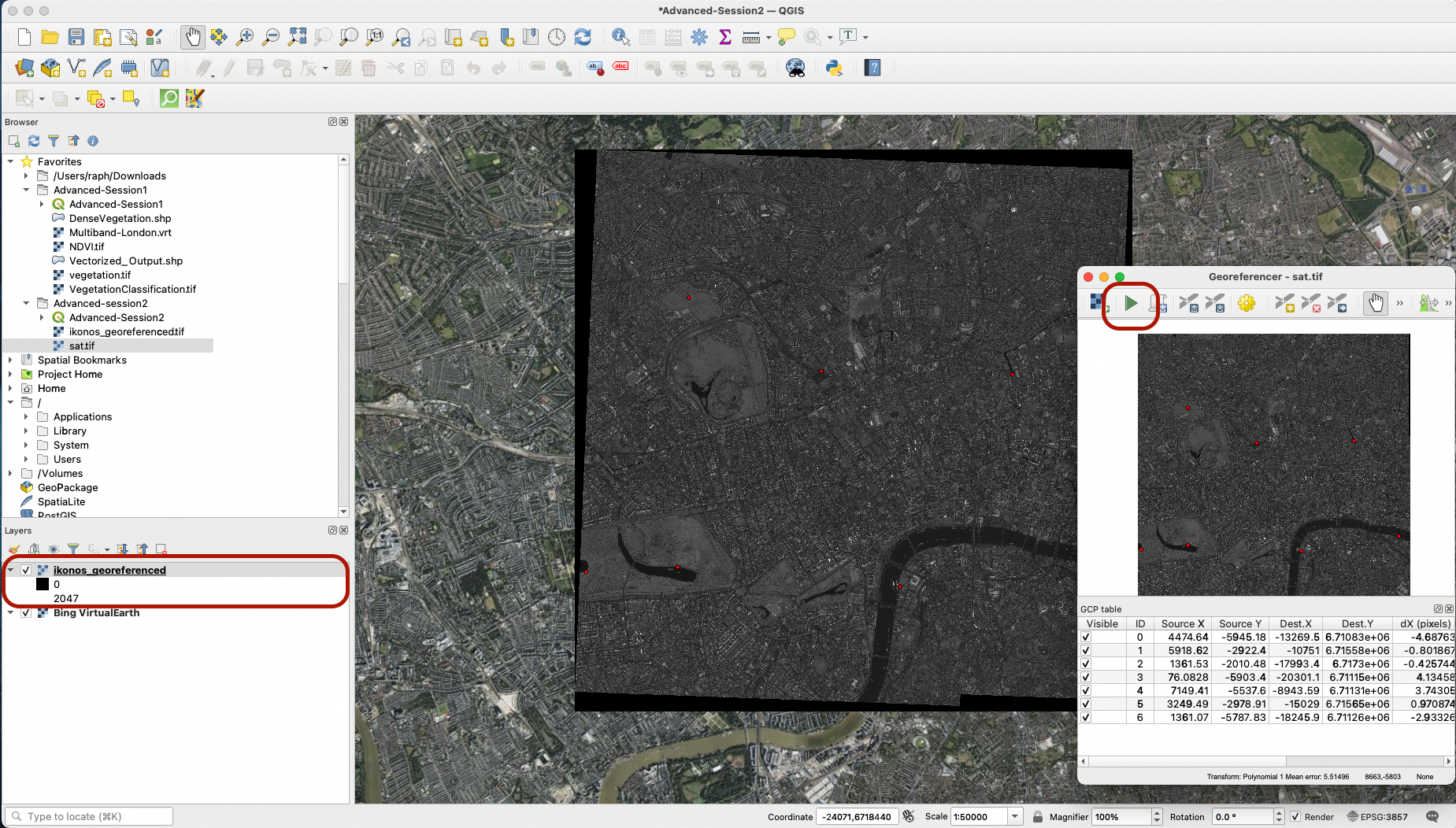
Once you’re happy with your GCPs, you can press the Start georeferencing button to launch the process and load your spatially referenced image onto your map canvas!

 

4.4 Exploring the georeferenced image

Explore the angles of your image, turn your layer on and off to see whether your georeferencing is accurate. If not, you can go back to your georeferencer and edit your GCPs. You could also, if you were working with another type of image and you noticed strong gaps, consider other transformation types that model different transformations across your image (this is especially useful if you work with old maps that can have slightly distorted boundaries or coastlines compared to reality).

 

V. Digitizing

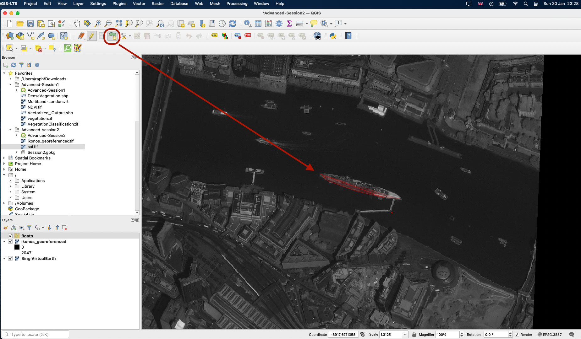
As a final step, let’s illustrate how you can create a vector layer uding the digitizing toolbox. Let’s imagine you want to create a dataset of the boats that were present on the Thames at the time the picture was taken.

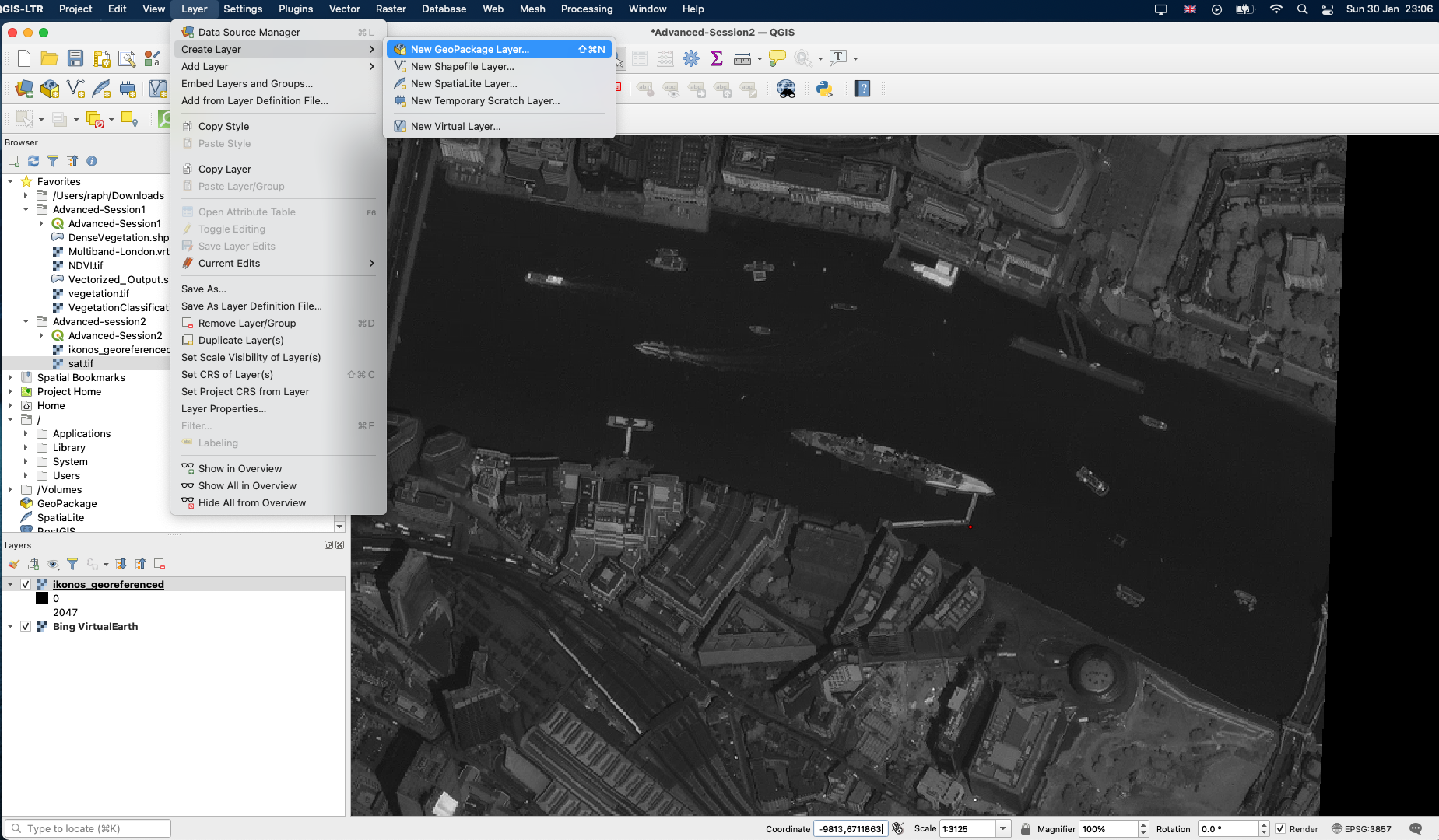
Navigate to the coordinates (-8906,6710902) to find the large boat in the London Bridge area. In your top menu, click Layer > Create new Geopackage layer.

 

Create a database location for your geopackage (I called mine Session2.gpkg and saved it in the Advanced-Session2 folder), give the layer a name and select Polygons as the Geometry type. Make sure the CRS is set to the Project CRS (EPSG:3857). You can then define the architecture of your attribute table by adding new fields. For instance we can add:

• a field Docked of type Boolean, where we will indicate if the boat is docked or not,
• a field Size of type Text data where we will indicate the size of the boat (small, medium, large).
• a field Year of type Date, which we will set to 2008 for all of these boats as our picture dates from 2008.

You can leave the Maximum length field empty each time and just press Add to Fields list to add your field to the table.

 

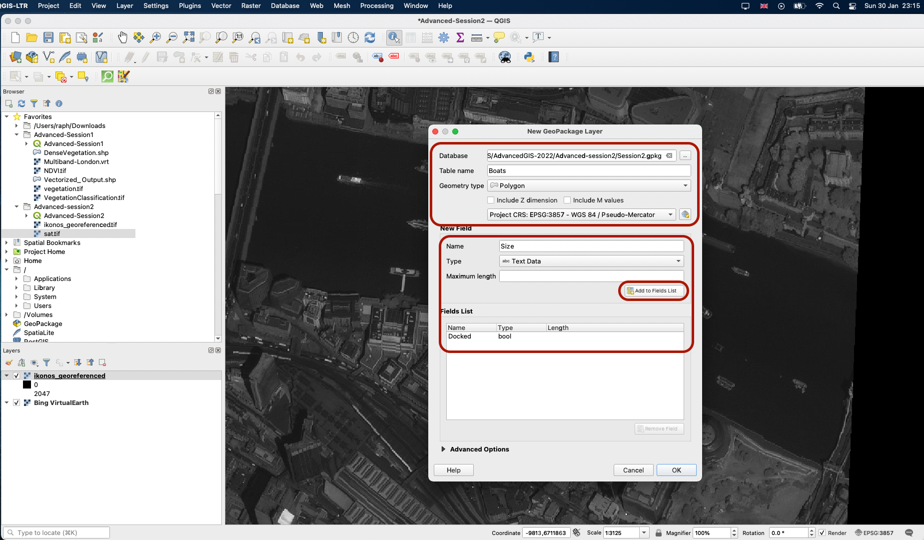
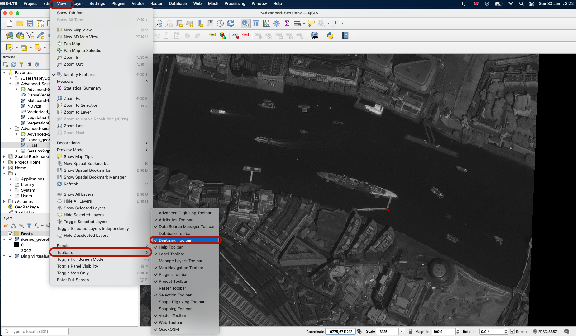
Once you have the three fields ready, you can press OK. A new Boats layer is created and appears in your Layer list panel. In yur top View panel > Toolbars, make your that your Digitizing toolbar is ticked. You will spot in in your top toolbars area.

 

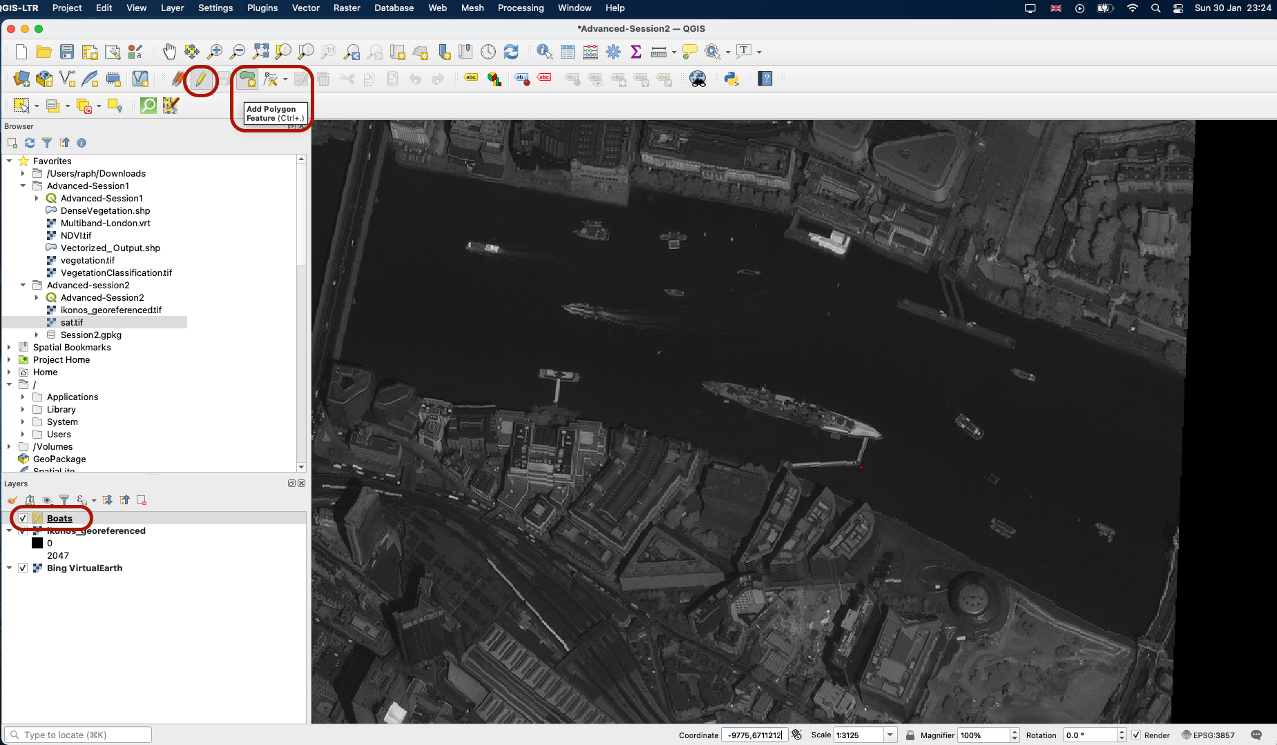
You can start an editing session by pressing the yellow pencil button (you can now make edits to the dataset!) - make sure you have selected Boats in your layer list before pressing the pencil; this is the layer you want to work on. You can then click on the green blob button to Add Polygon feature.

 

Draw the contours of the boat by clicking on its vertices.

 

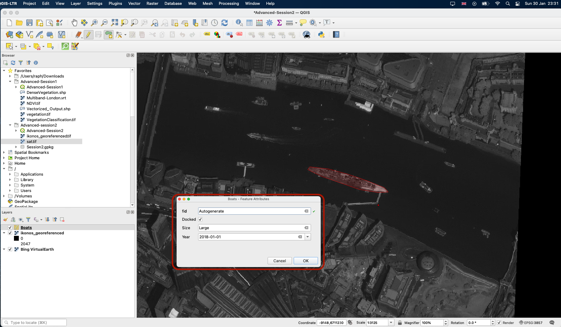
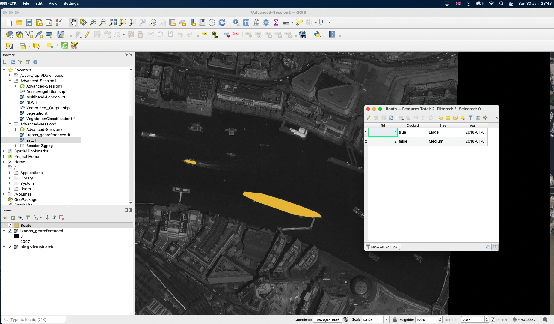
When you’ve positioned your last point, right click and a pop up window will ask you to fill the values of the attribute table. Leave fid to Autogenerate, tick the Docked checkbox because this boat is indeed docked, set the size to Large and the date to 2018-01-01.

 

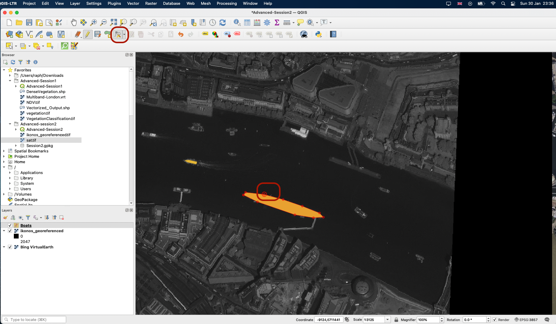
Press OK; your polygon is now part of your dataset! Try to repeat the process with another boat. If you are not satisfied with the boundaries of one of your polygons, use the Vertex tool to edit the position of the points!

 

When you are done, you can press the yellow pencil button to close your editing session and save your changes.

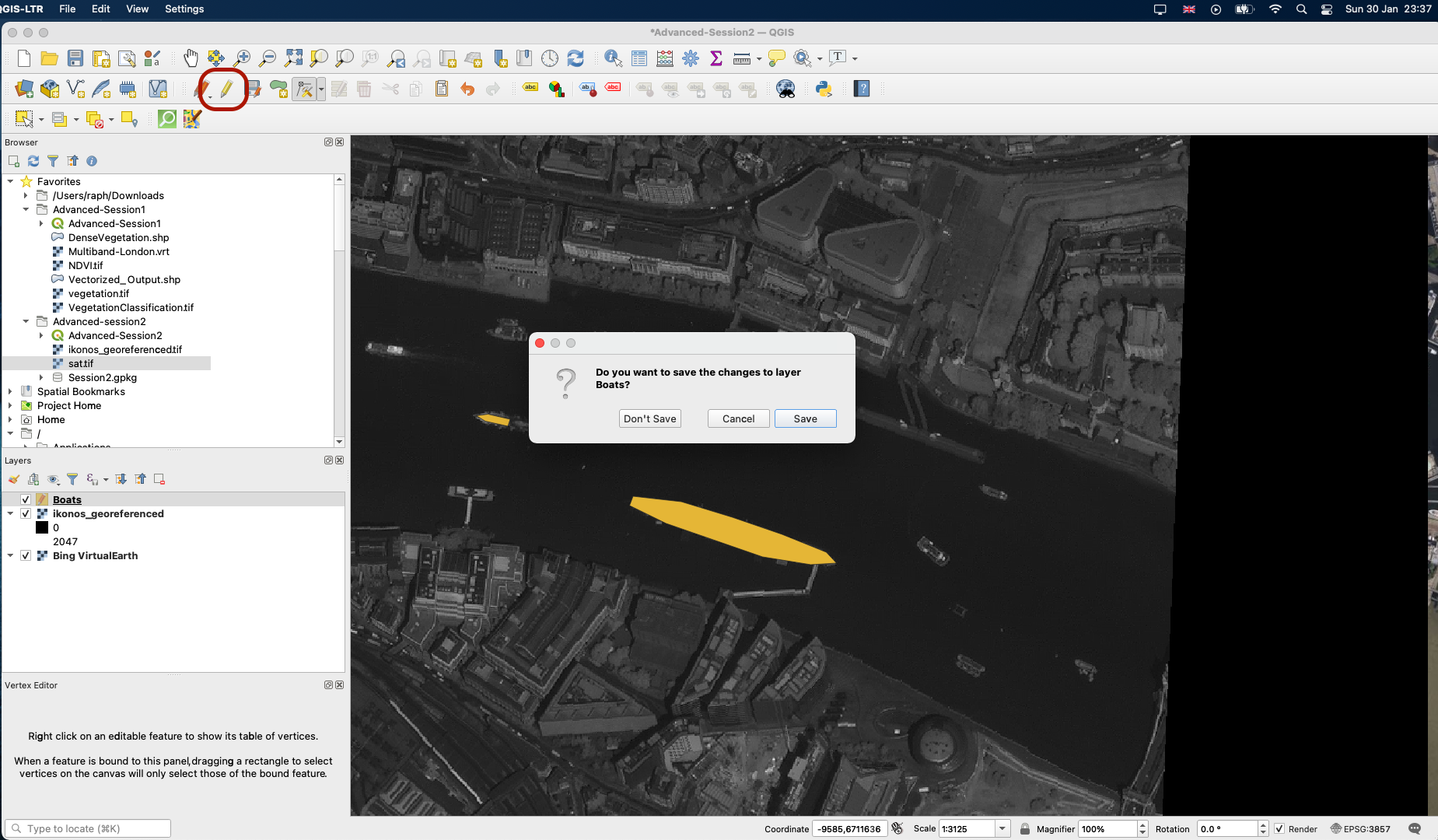
  Now if you open the attribute table of the Boats layer, you’ll find that it contains the data you have just created and has generated unique id in the first column. You can always reopen the editing session and add more boats, edit or remove existing ones or their attribute table.

 

 

To go further, you can experiment digitizing other types of features (lines for roads, points). For example, you can digitize the position of certain trees in the parks, or of footpaths. You can also digitize features from the satellite imagery basemap, which is more recent than our georeferenced image.

 

Congrats, you have successfully completed this tutorial!

 

 

Next Tutorial >

Back to the syllabus >