Session 3 - Bivariate Choropleths
23 Jan 2022Advanced GIS · Sciences Po Urban School
Lecturer: Raphaëlle Roffo
I. Session 3 Overview
Download the slides
- Additional raster dataset examples
- Bivariate choropleths
II. Tutorial
Goals:
- Creating a bivariate choropleth
Download the data
Create an Advanced-Session3 folder, and download the following data in this folder. Add the folder to your Favourites in QGIS to have an easy access to it.
- Census: Census data for the Greater London Metropolitan Area. It’s comes as a CSV file (tabular,non-geographic data) and comes at the LSOA level. Choose the
Current LSOA boundaries post-2011file in CSV format (NOT as.xlsx!). If when you clickDownloadyou land on a page that looks like this, simply pressCtrl + Sor⌘ + Sto save the file, and make sure you give it a.csvextension.

-
LSOA Boundaries for England & Wales: Lower Super Output Areas (LSOA), the smallest census unit in the UK, like the IRIS zones in France. A few versions are available but we will use the Boundaries Generalised Clipped (BGC) dataset, where the boundaries of each polygons have been generalised to 20 meters, resulting in a less heavy dataset without major information loss. Click
Downloadand download the dataset as GeoJSON (or Shapefile). -
But because the LSOA dataset is national and our Census data is limited to Greater London, we need the Greater London boundaries. They will allow us to select the LSOAs that are within the Greater London Metropolitan Area. Download the data as zipped Shapefile.
III. Data import and pre-processing
3.1 Set up the project: Try it on your own!
The first steps of this tutorial are similar to the Intro to GIS Session 6 tutorial. Try to carry out these steps by yourself to test your skills!
- Open a new blank project
- Drag and drop the LSOA-level census dataset as CSV, the LSOA boundaries for England & Wales, and the Greater London boundaries onto your map canvas
- Clip the LSOA layer to the shape of Greater London, so as to only keep the polygons that fall in Greater London.
- Join the census table onto your Greater London LSOA polygons.
If you get stuck, don’t panic as the following section walks you through this process.
3.2 Set up the project: Solution
3.2.1 Project setup
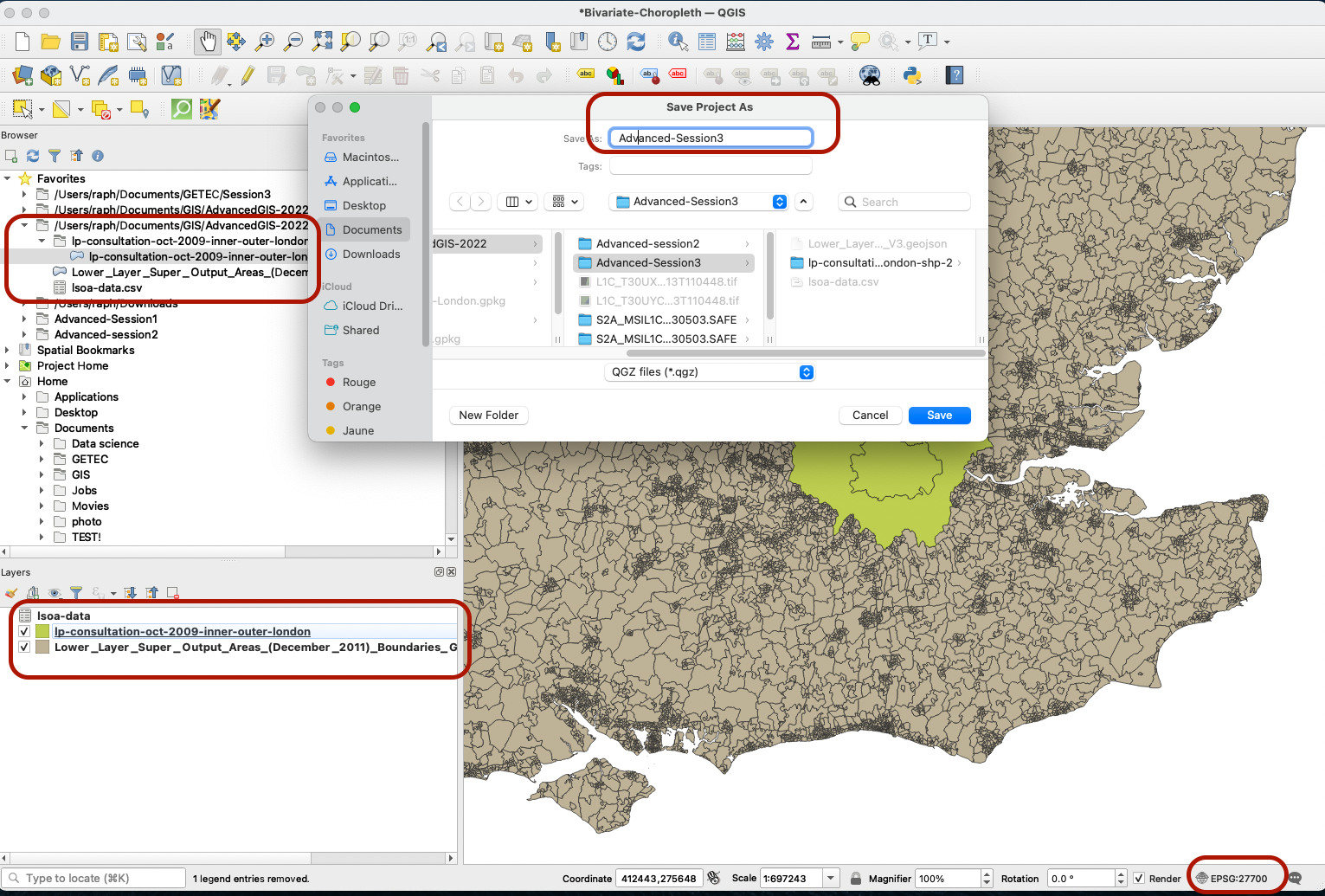
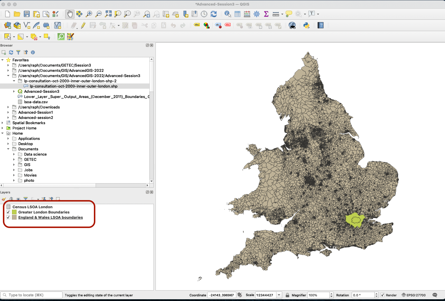
Open a blank QGIS project. Make sure the CRS is set to EPSG:27700, then drag and drop your Census CSV file, LSOA boundaries and Greater London boundaries onto your map canvas. Save your project as a QGZ file for now, for instance Advanced-Session3.qgz. Remember to save your changes often using the flapdisk icon.
First, for improved clarity, let’s rename our layers to make navigation easier:
- Rename
lp-consultation-oct-2009-inner-outer-londontoGreater London Boundaries. - Rename
Lower_Layer_Super_Output_Areas_(December_2011)_Boundaries_Generalised_Clipped_(BGC)_EW_V3toEngland & Wales LSOA boundaries - Rename
lsoa-datatoCensus LSOA London
Now, what we want ultimately is a single polygon layer that contains census data at the LSOA level, and covers the Greater London extent.
But notice that, while we are only interested in the Greater London Metropolitan Area (GLMA) and only have census data for that region, the LSOA file we downloaded covers the whole of England & Wales. If we tried running the join between the LSOA boundaries layer and our census table, it may take a very long time to run due to the large number (34 753!) of features in the boundaries layer (= 34 753 rows in the attribute table).
That’s why in this case and more generally speaking, it can be a good idea to only keep the features of the geographic area you’re interested in before running slightly intensive algorithms such as table joins or geoprocessing. This will speed up the processing time for the following steps.
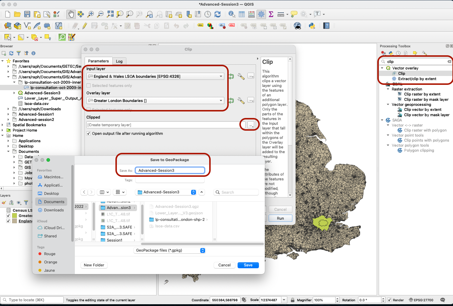
3.2.2 Clipping the LSOA to Greater London extent
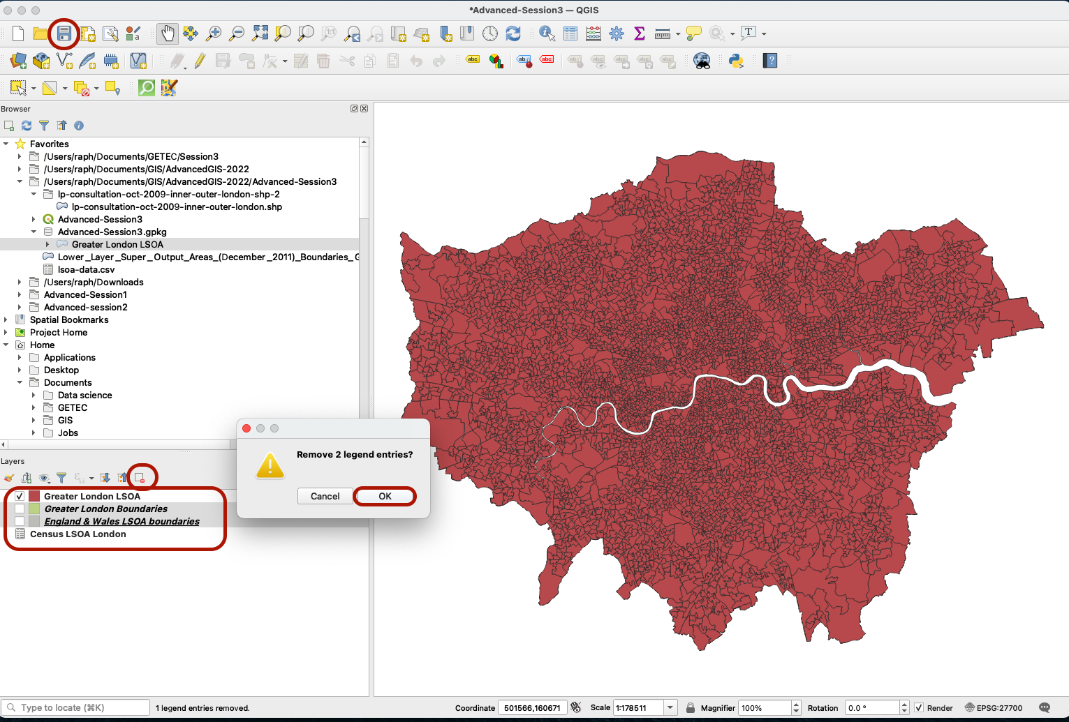
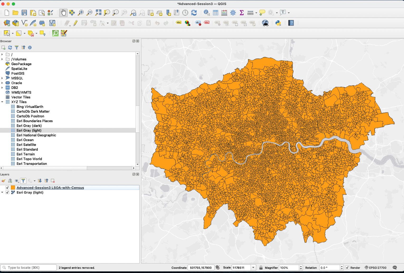
First, we want to create a subset of the LSOA layer that only contains LSOAs in the GLMA. Use the Clip tool to get a neat, cookie-cutter like selection of LSOAs within the GLMA boundaries. Find the Clip in your Processing toolbox and set it up to clip your LSOAs to the shape of Greater London Boundaries. Set the output to be saved as a geopackage layer. You can call this geopackage Advanced-Session3 and then the layer to be called Greater London LSOA. Press Run.
You can now remove the England & Wales LSOA Boundaries and Greater London Boundaries layers from your map canvas, and save the changes.
3.2.3 Joining the census data onto the LSOA polygons
The census data comes as a non-spatial table. We want to combine information from that table and the geographic boundaries of the LSOAs into a single dataset, using a table join.
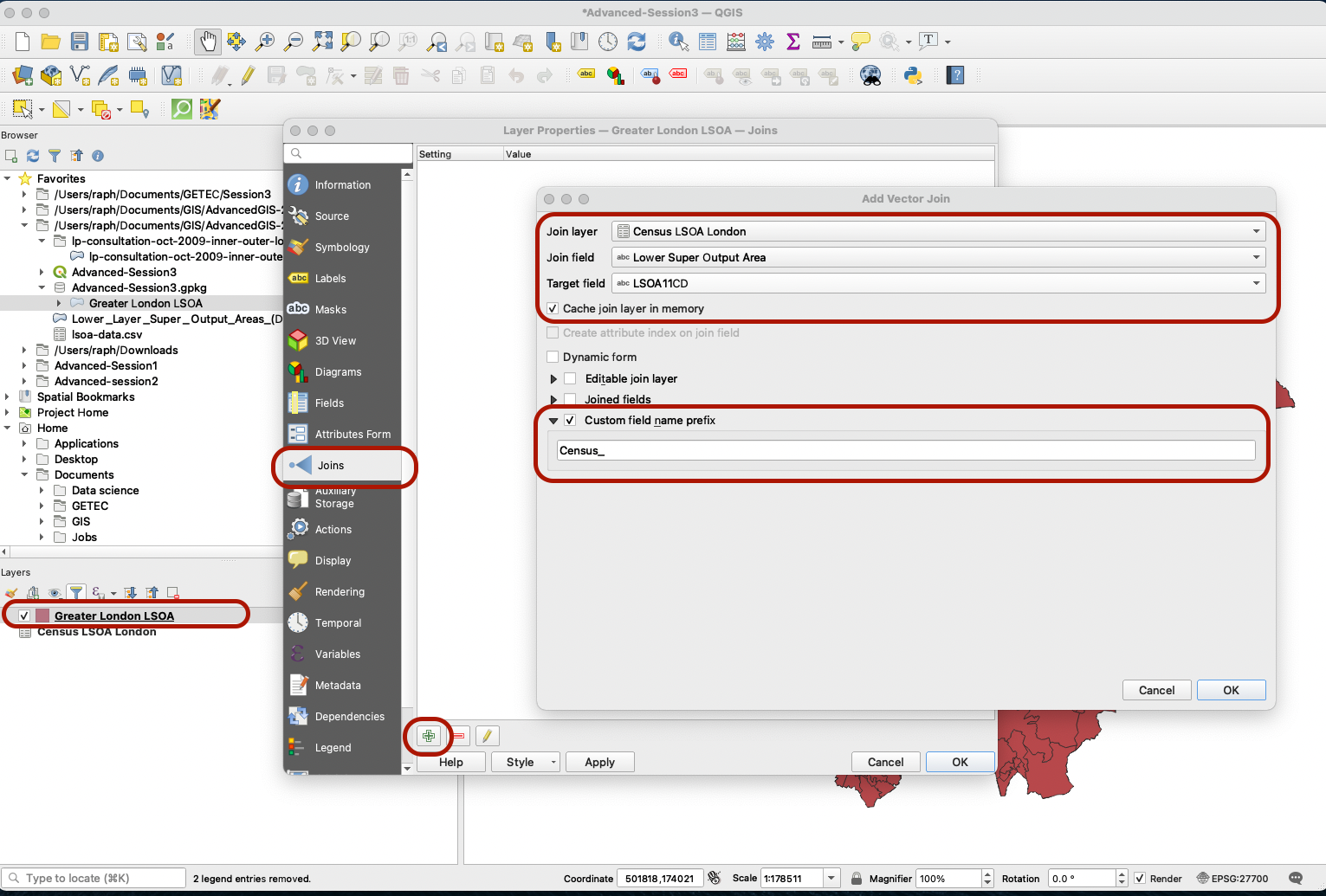
If we look at the attribute table for theGreater London LSOA layer, it contains the LSOAs in Greater London, with some basic information and a column with a unique identifier for each LSOA: the LSOA11CD column.
If we look at the attribute table for the Census LSOA London table, it contains a lot of variables but also a Lower Super Output Area column which contains very similar codes to LSOA11CD. This is the official LSOA code, produced by the Office for National Statistics (ONS). After a couple quick checks (comparing Names and Codes in both table), we confirm that they are indeed the same codes in both tables.
Note that the LSOA11NM and Names columns would also seem to be good matches as Key fields for the join; however names are more prone to spelling differences (a space or apostrophe might be present in one table and not the other). That’s why when available, you should alwyays opt for the standardised code instead!

Double-click the Greater London LSOA layer to access the Layers properties, navigate to the Joins tab and click the Green Plus sign to create a new join based on those two fields. You can edit the custom prefix to be shorter, for instance Census_.
Press OK in that window, then OK again to close the Layer properties. If you open your attribute table you will now see the additional fields for taht layer.
Now can be a good time to save a copy of this “super” LSOA Census layer in your geopackage. Right-click your London LSOA layer, Export > Save Features as... , save it in your Advanced-Session3 geopackage and give it a descriptive name, for instance LSOA-with-Census. Make sure the CRS is British National Grid. You can then remove the two other layers. You can also import a basemap as backdrop to your project. If you do not have basemaps under the XYZ Tiles section of your browser, refer to the Intro to GIS Session 3 tutorial to set it up.
3.2.4. Fixing the data type
Now that our data is ready, it’s time to explore the variables and find two variables that we could cross in the bivariate choropleth. Here, we choose to explore how the Census_Car or van availability;Cars per household;2011 and Census_Public Transport Accessibility Levels (2014);Average Score; variables interact across London. Our hypothesis is that richer area, where a larger number or households own a car, are also well connected to public transport (in areas such as Westminster and Kensington), and that poorer area have less access to public transport while simultaneously having low car ownership rates. But what is the situation like in the more remote boroughs of Greater London?
-
The Cars per household is an average rate based on car ownership in the LSOA.
-
Public Transport Accessibility Levels is a score ranging from 0 to 6b, where a score of 0, 1a or 1b is very poor access to public transport, and 6a or 6b is excellent access to public transport. The score in this column reflects the average score of household in that LSOA. Due to the deduplication of 1a/1b and 6a/6b, the data in this field actually ranges from 0 to 8:
- 0,1,2 = Scores of 0, 1a or 1b = Poor access
- 3, 4, 5 = Scores or 2, 3, 4 = Average access
- 6, 7, 8 = Scores of 5, 6a, 6b = Good access
However, if you observe your Fields in the Layer Properties, you will notice that these two fields are stored as String and are not being read by QGIS as figures. This is problematic because we cannot build a choropleth with categorical data, we need continuous, decimal numbers.
You could use the Field Calculator to add new columns that are a copy of these fields, except in real numbers format. This time, try to use the Refactor Fields tool instead. This tool allows you to batch edit the attribute table. You can for instance choose to only keep the fields you are interested in, and save them as real numbers. Make sure to keep all the fields that came from your boundary layer (fields 1 to 11), and to only remove the fields from the census that you are not interested in.
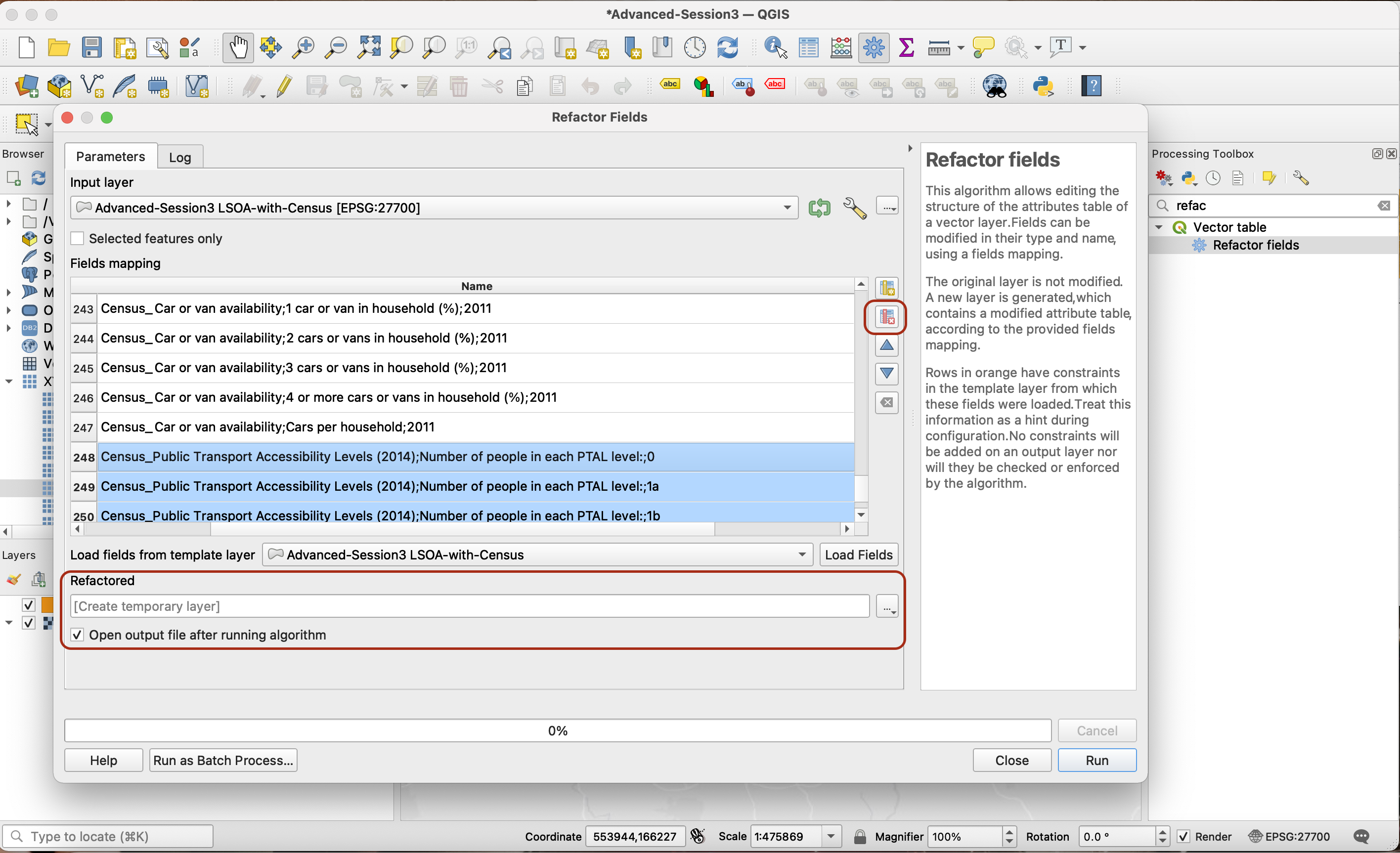

You now have a dataset that is less heavy, and contains exactly the two columns you want, in the right data format.
IV. Building the choropleth
4.1 Reclassifying the data
The first step is to define, for each of these variables, how to cut the distribution into 3 categories: low, medium and high.
For Cars/household:
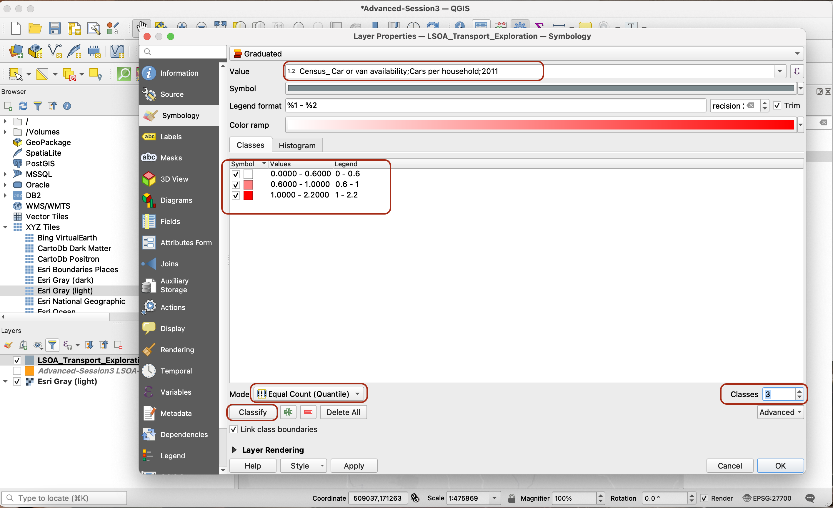
Go into your Layer Properties > Symbology tab. Pick the style Graduated and select your Census_Car or van availability;Cars per household;2011 variable. We will use quantiles as classification method, with only 3 classes. Now, make note of the break points between each of those classes: 0-0.6, 0.6-1, 1-2.2
Now go into your Fields, open an editing session by clicking on the yellow pencil, and click on the field calculator to calculate a new field of type Integer.
You are going to reclassify your values into three categories so that the bottom 33% car ownership values get assigned the value of 1, the middle 33% a value of 2 and the top 33% a value of 3:
CASE WHEN  "Census_Car or van availability;Cars per household;2011" <= 0.6 THEN 1
    WHEN "Census_Car or van availability;Cars per household;2011" > 0.6 AND "Census_Car or van availability;Cars per household;2011" < 1 THEN 2
    ELSE 3
END

For Transport Accessibility:
For Transport Accessibility, our PTAL scores already give us an indication of the level of access. Rememebr that the data ranges from 0 to 6b and due to the deduplication of 1a/1b and 6a/6b, the data can actually be classified as follows:
- 0,1,2 = Scores of 0, 1a or 1b = Poor access
- 3, 4, 5 = Scores or 2, 3, 4 = Average access
- 6, 7, 8 = Scores of 5, 6a, 6b = Good access
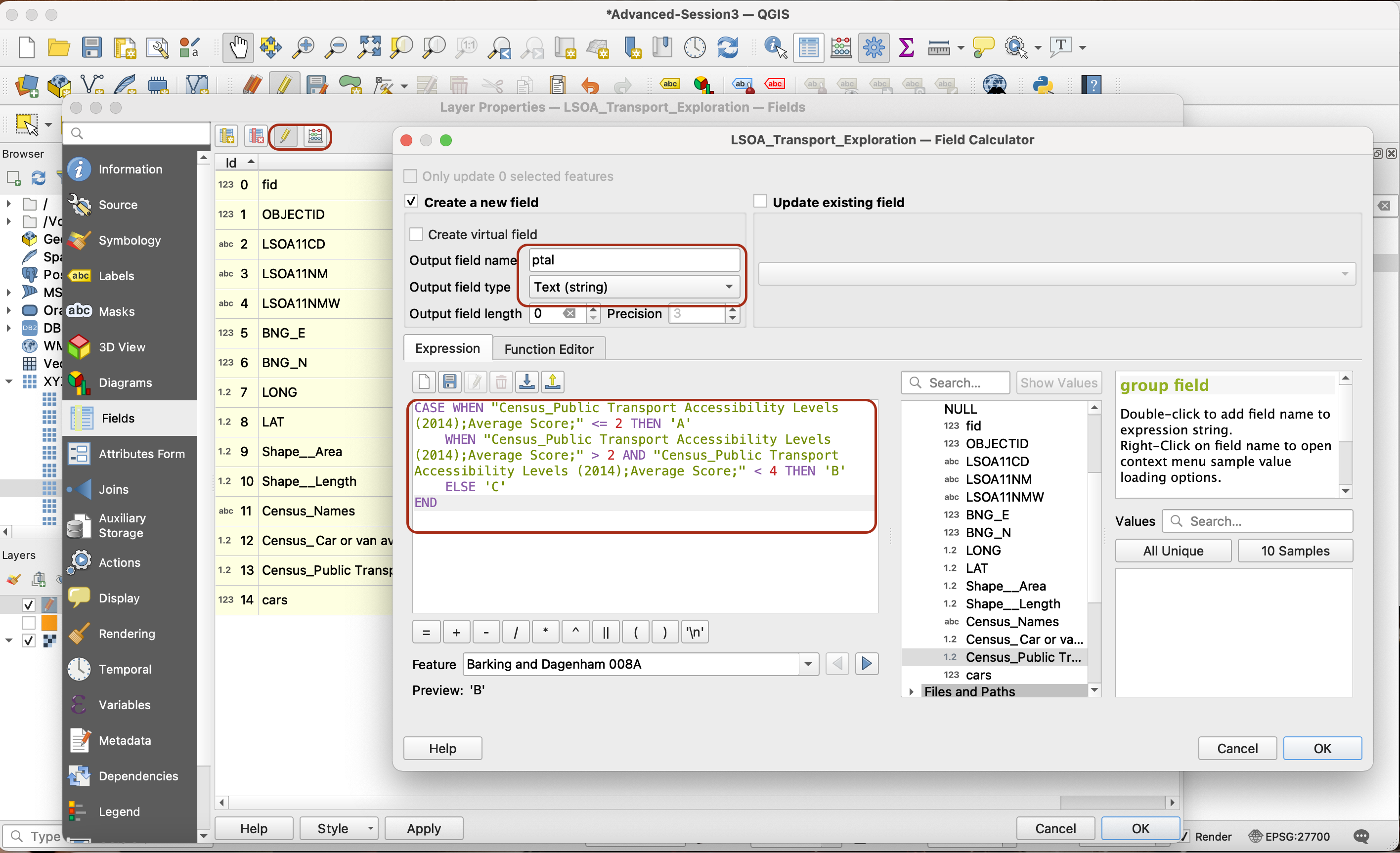
Using the field calculator we can directly create a new field called ptal, of data type String, and enter the below expression:
CASE WHEN "Census_Public Transport Accessibility Levels (2014);Average Score;" <= 2 THEN 'A'
    WHEN "Census_Public Transport Accessibility Levels (2014);Average Score;" > 2 AND "Census_Public Transport Accessibility Levels (2014);Average Score;" < 4 THEN 'B'
    ELSE 'C'
END
4.2. Combining the two reclassified variables as a single bivariate class
Now you can combine these two reclassified groups to come up with a combination of 3x3=9 possible options: A1, A2, A3, B1, B2, B3, C1, C2 and C3. To do so, using the field calculator create one last new field called bivariate, of type String. Then use the concatenate function to “paste” the values of cars (as a string) and ptal in a single new field:
concat("ptal",tostring("cars"))
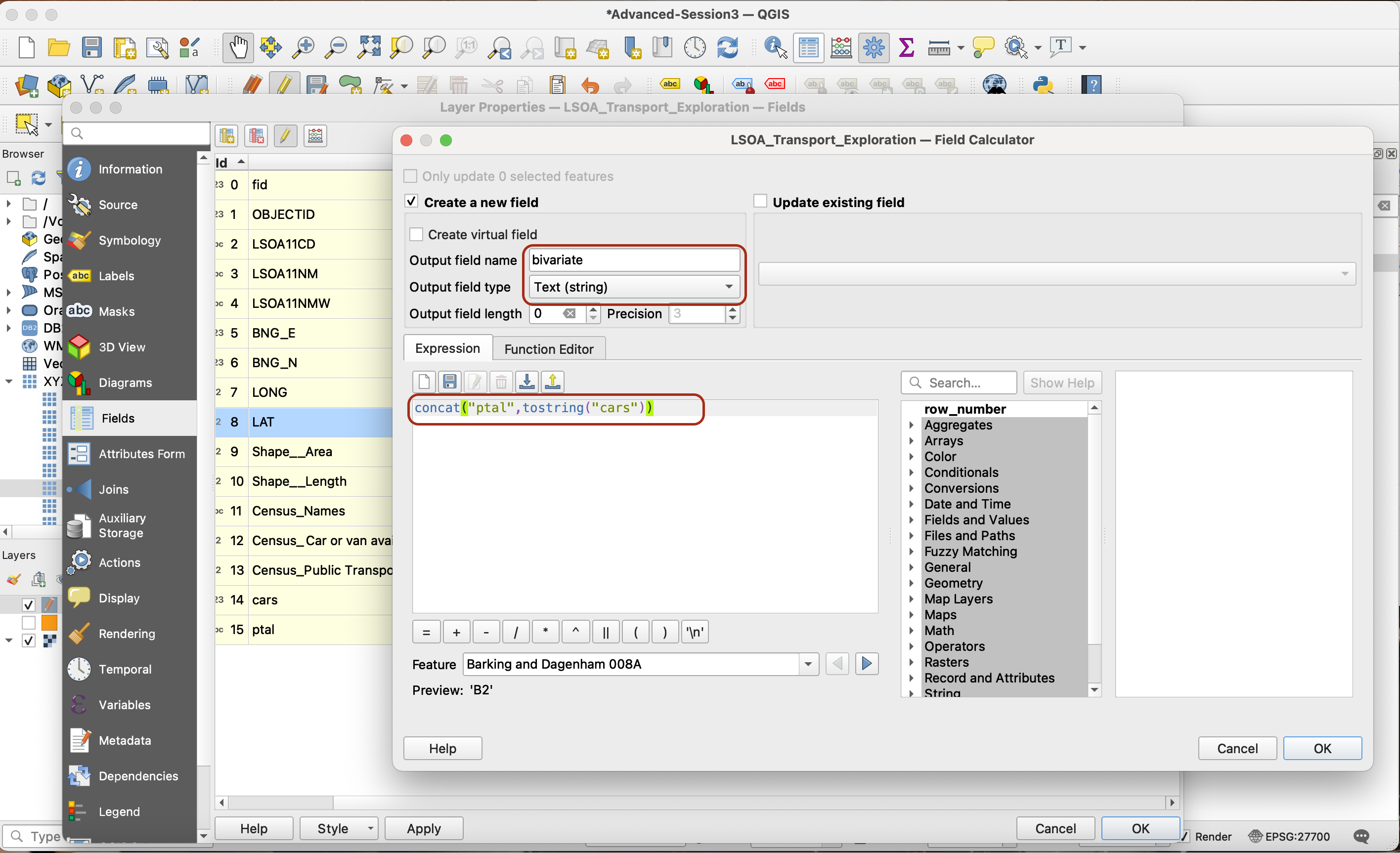
Save your edits by pressing the yellow pencil and saving the changes. You now have a column bivariate ready to use!

4.3 Symbology
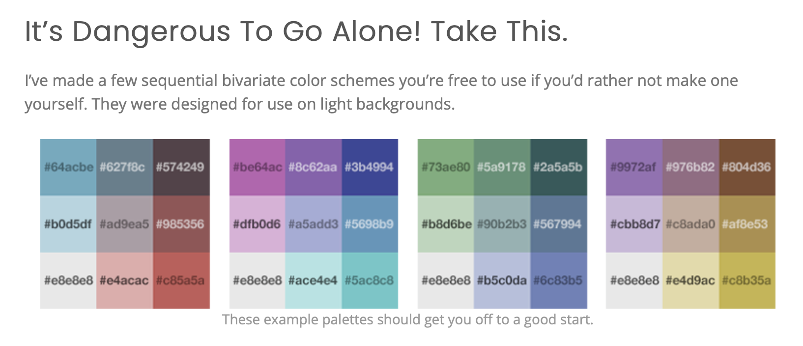
The final step in this process is to build your symbology. Pick one of the palettes designed by Joshua Stevenson in this article:
Go to your Symbology tab and select Categorized symbology. Pick bivariate as your variable (you may need to scroll a bit down the list of variables). Click Classify to bring up all the values. You can delete the extra row without value using the red Minus sign.
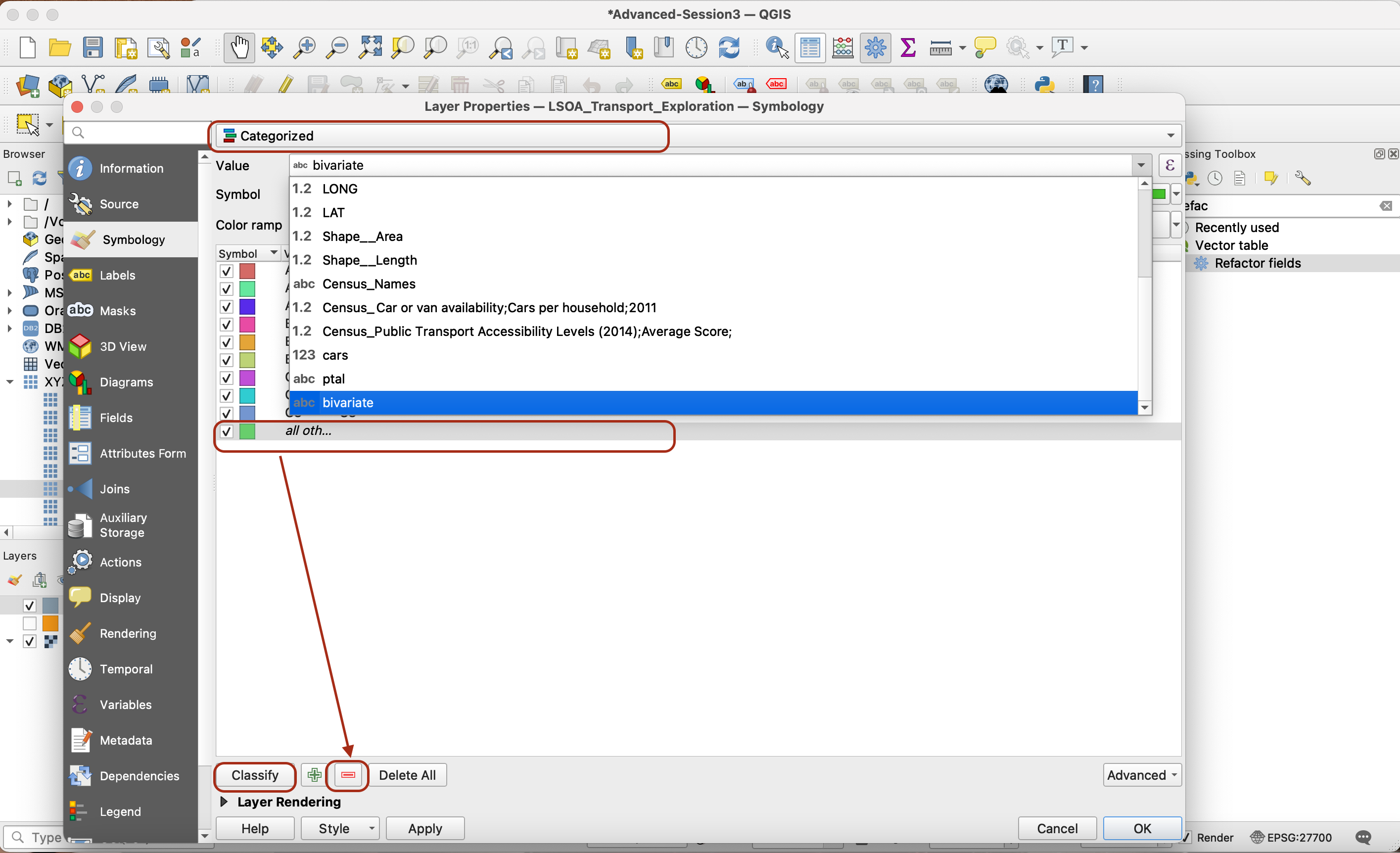
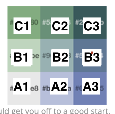
Now our values starting with A have a low Public Transport Accessibility Level, and those ending with 1 have a low car ownership level. Whichever colour scheme you picked, we are using the bottom left corner of the colour matrix as the A1 value and the darkest, top right corner as C3.
On your colour ramp, click on each colour individually and use the rgb code to edit the colour to the exact one you need:

As a final step, click on the overarching symbol, then on its Fill properties to make the polygon stroke transparent.

4.4 Results
Congrats, you have successfully created your first bivariate choropleth!

The map we obtain is in line with the hypothesis we initially formulated. In wealthier areas of West London, the car ownership rate is high and simultaneously the public transportation levels are very high. This is in sharp contrast with East London, for instance in the Tower Hamlets area, where mobility seems to be very limited. In the outskirts of Greater London, car ownership rates are quite logically high as the public transportation offer gets very limited.

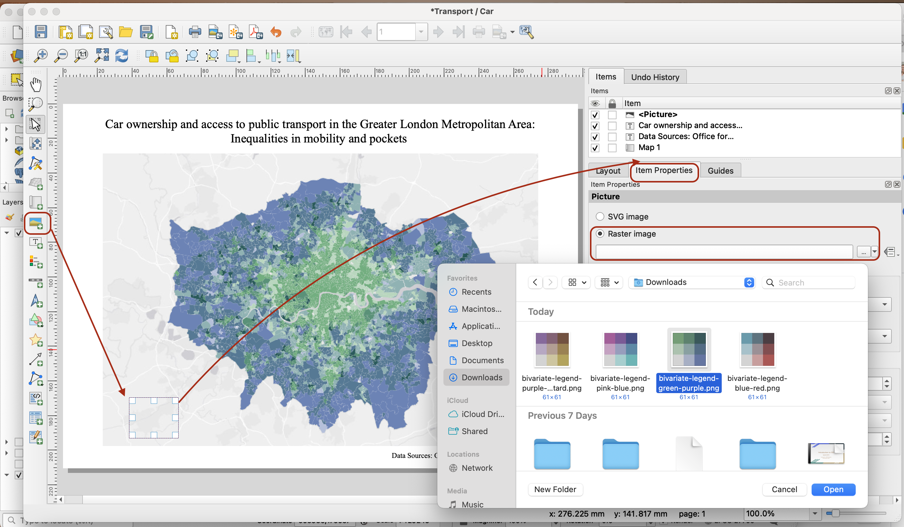
4.5 Map export
As a final step, try and produce a map export using the layout composer.
For the legend, I have created one legend block for each of the four colour schemes. Save them in your GIS folder by right-clicking the images below.


You can now simply import them as images in your print layout and use arrows to build a minimalistic legend.
If you have your own colour scheme and want to create your own, you can use the bivariate plugin in QGIS. If you go down that route, you will have to follow the steps used for creating the legend in this tutorial. You may also simply use a graphic design software of your choice.
Then you can use arrows and other map elements to create a beautiful map export.
Congrats, you have successfully completed this tutorial! Try replicating this analysis with other variables of your choice, or pushing this analysis further.
Final note:
If you wanted to build a bivariate choropleth in R using ggplot and sf, you could do so by following this great tutorial.