Session 3 - Working with vector data & the attribute table
16 Nov 2021Introduction to GIS · Sciences Po Urban School
Lecturer: Raphaëlle Roffo
I. Session 3 Overview
Download the slides
- Understanding the attribute table
- Querying data based on their attributes
- Joining layers: why and how?
II. Tutorial
Goals:
- Load basemaps
- Access summary statistics about a field
- Understand the attribute table
- Explore how features and records are related
- Create a point layer from a
*.csvfile - Create a table join
- Create a query to select features by attribute
- Use queries to only display a subset of your layer’s features
Data:
You can find the geopackage for this session here and the Schools CSV file here (right click anywhere on the page and Save as... to save it as Schools.csv in your folder).
Save both in your documents (again, avoid saving in Dropbox/Cloud folders as it may get QGIS very cranky) under a Session3 folder.
III. Setting up
Open the project
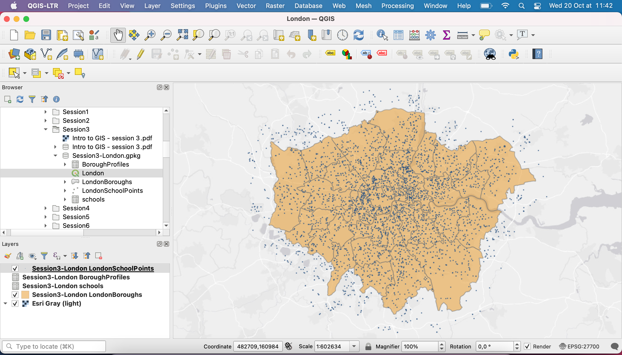
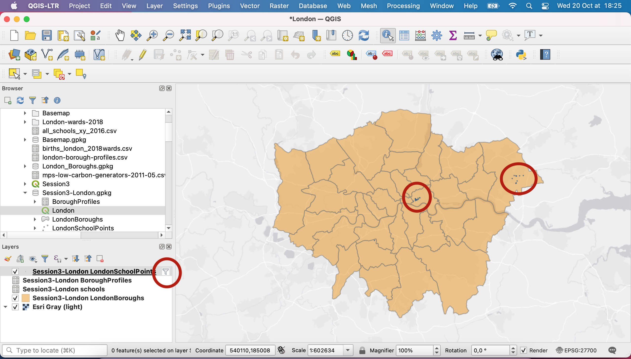
Open QGIS, and open a blank document. In your Browser panel, navigate to this Session3 folder. Click the arrow to see the content of the geopackage. Double click the London project file. Data for this project come from the London Datastore. This should automatically load these layers using the same symbology as in this screenshot. You may not have access to the basemap however. QGIS may give you an error message, which you can ignore for now.
To load the basemap, we’re going to use Python.
Load basemaps
One way to add basemaps in QGIS is to connect to a tile service from some online server. You can do that very quickly using the Python console! Visit this link. Select & copy the entire text on that page (press Ctrl+A or ⌘+A, then Ctrl+C or ⌘+C).
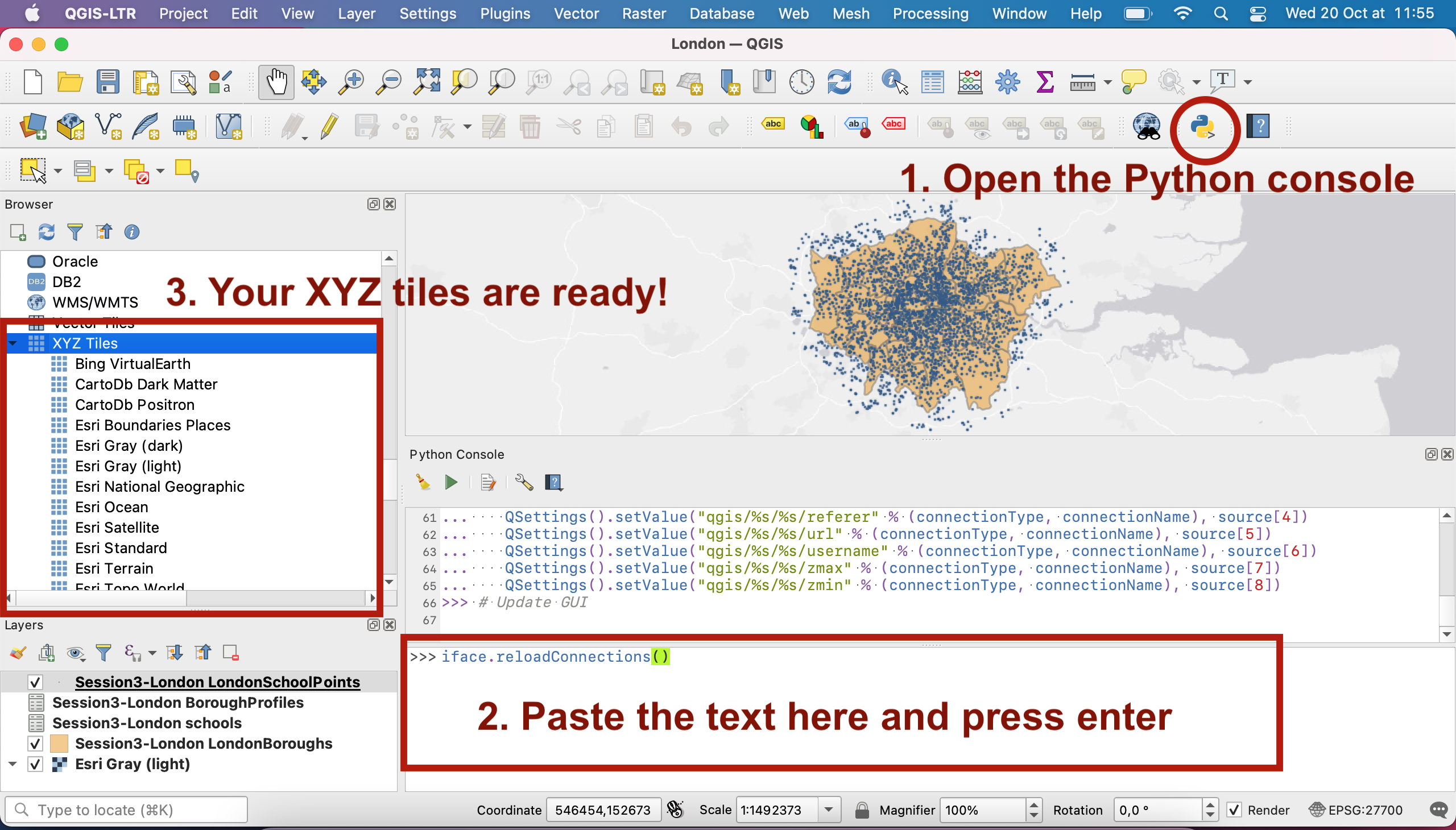
Now go back to QGIS, and open the Python Console by clicking the Python icon in your toolbar, or going to your Plugins Menu > Python Console. This opens a new panel, usually located below your map canvas. Simply paste the script that you just copied (Ctrl + V or ⌘+V) and press enter. That’s it!
Now if you look into your Browser panel and scroll down, you will see a XYZ tiles section. Click to open and you’ll see a list of basemaps ready to use! You can close the Python console. Note that you only need to create this connection once, and the basemaps will now always be available in your QGIS console even when you work on a different project.
You can drag and drop the basemap you like onto your canvas. In this case I have used Esri Gray (light) because its design is quite simple and not overwhelming.
IV. The statistics summary panel
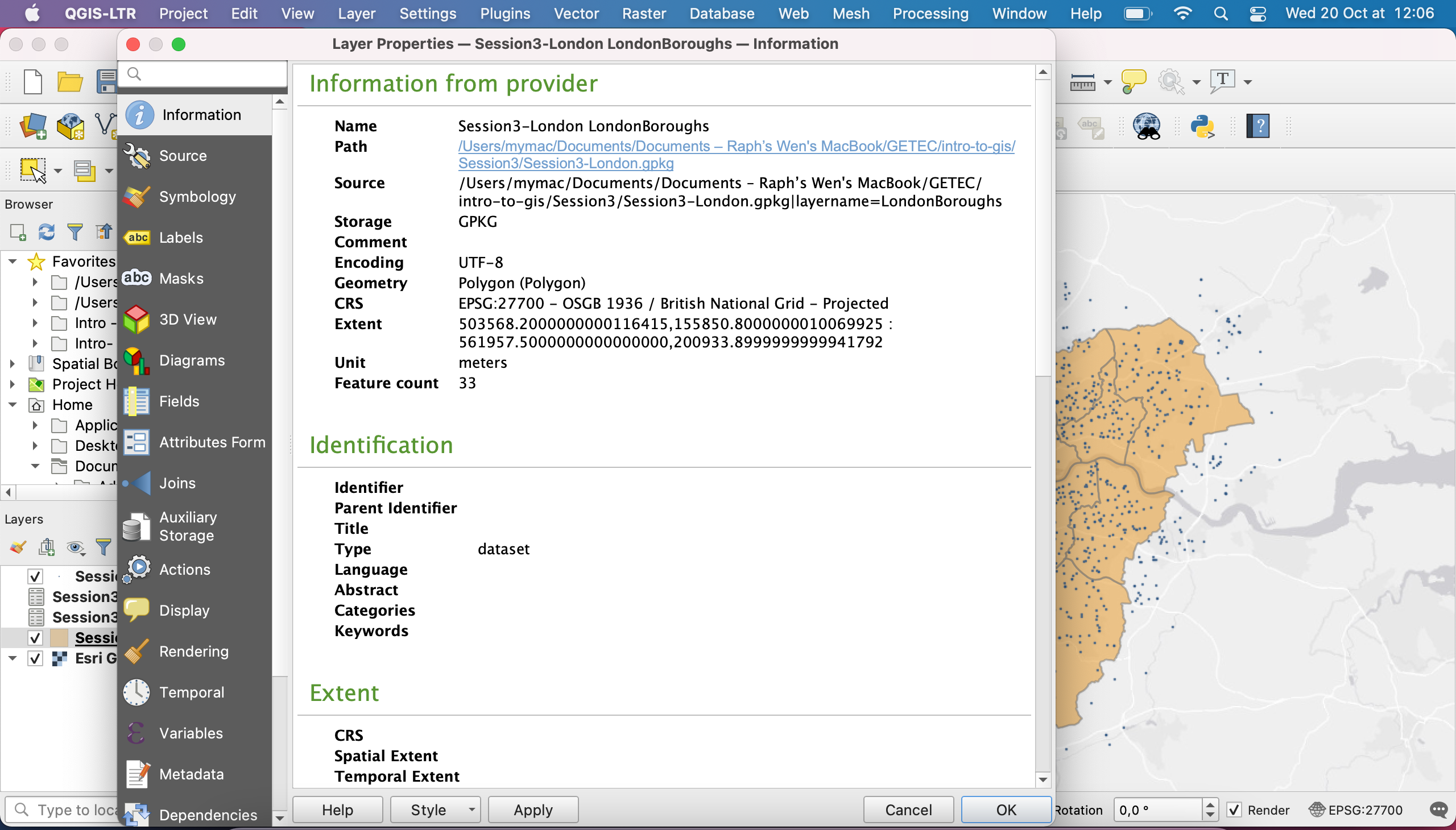
As a means of exploring a layer, you may want to see some form of summary. Let’s have a look at the LondonBoroughs layer. In your Layers panel, double-click the LondonBoroughs layer or right-click > Properties.... This opens up a very important menu from which you can access a LOT of useful tools to deal with your layer.
The first tab Information gives you some basic details about the layer: what’s the path to the actual dataset on your computer, what format is it in (geopackage), the encoding, the type of layer (Polygon), the Coordinate Reference System (British NAtional Grid), the extent (maximum x and y coordinates, so basically the bounding box that contains your layer), the unit (meters) and the feature count (how many polygons=features are there in this layer, whcih is equivalent to asking how many rows=records in the attribute table).
Close this menu and press Ctrl+6 or ⌘+6 , or navigate to your menu View > Panels > tick Statistics. A new menu appears. It’s a bit squished in the bottom left corner so I will undock it (click the top of the panel, drag it towards your map canvas) and make it a bit larger. I then select the LondonBoroughs layer, and pick a field I’m interested in. For example, I’m curious to look at summary statistics about the average land size for the London boroughs.
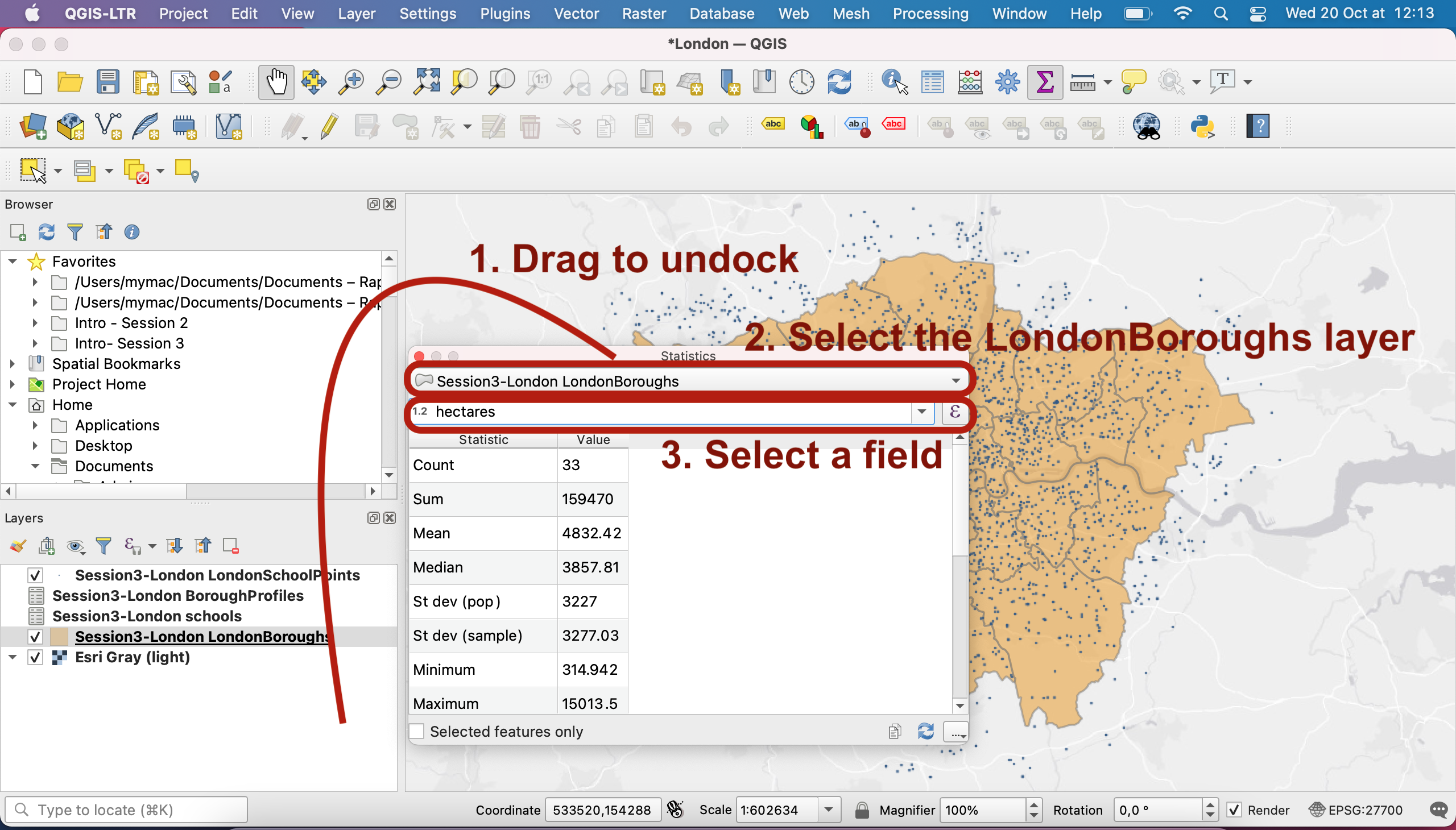
Indeed, we observe that there is huge variance in the size of these boroughs, between 315 hectares and 15,000 hectares. The median size is 3,857 hectares.
Try and expore other summary statistics, for example for the LondonBoroughProfile table and look at the demographic fields.
V. The attribute table
As seen in the lecture, the attribute table contains records for all the features present in a vector layer. Let’s see in practice what this means for the LondonBoroughs layer.
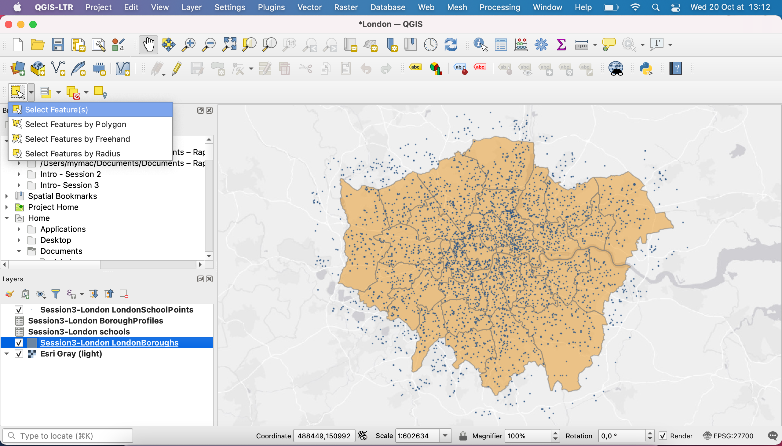
Click the LondonBoroughs layer in your Layers panel so its selected (blue). You have now access, in your toolbar, to the Selection tools. Use Select feature(s) and click on one polygon; it turns yellow. Now press your Ctrl/⌘ key or shift key to select a few polygons at once. The features that are added to your selection turn yellow.
Now open your attribute table (right click on LondonBoroughs in your Layers panel > Open attribute table, or click the icon in your toolbar). You will notice that some rows are highlighted in blue. They are the recors linked to your feature selection.
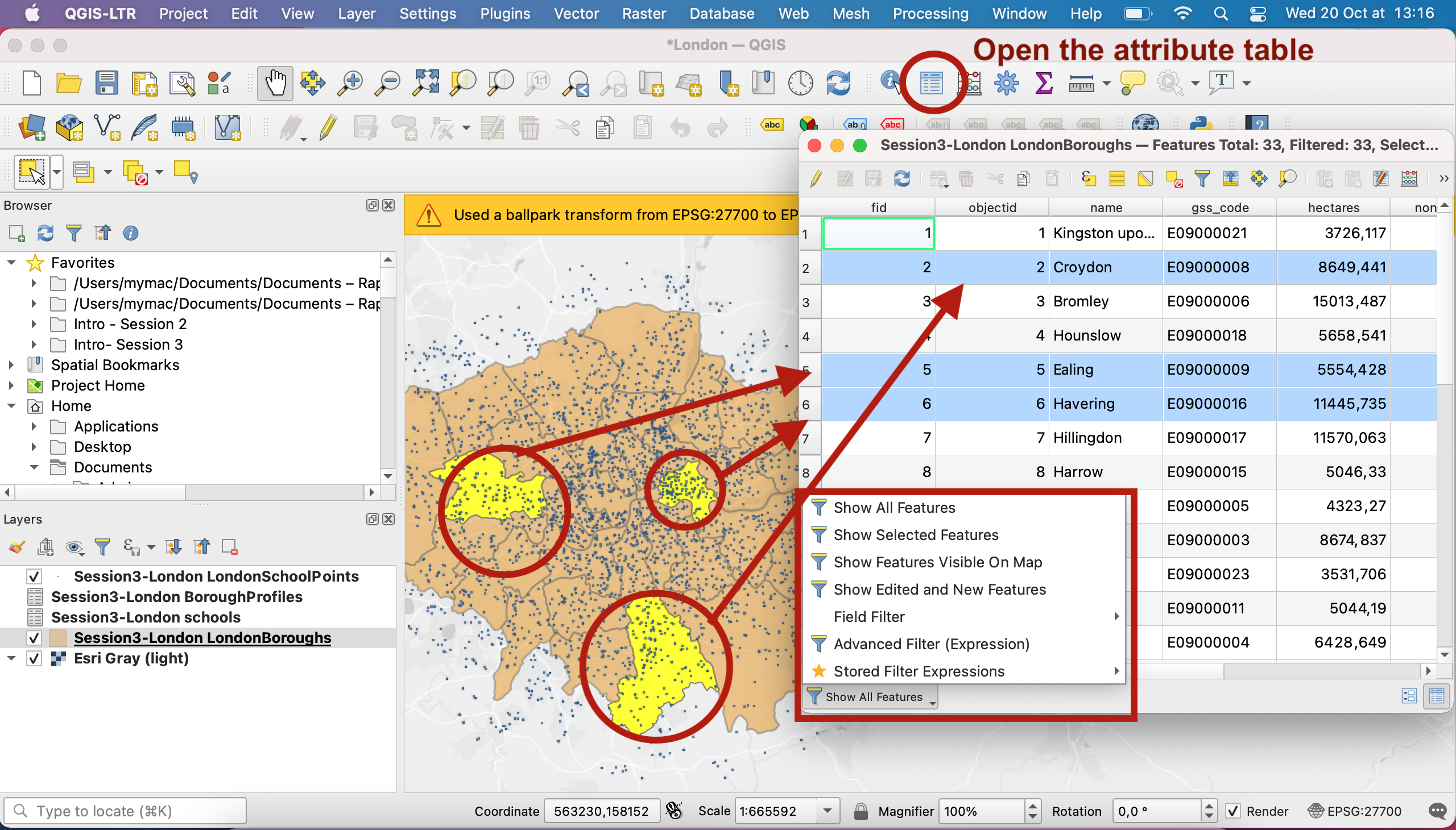
If you click on the bottom left filter, you can change the view; you could choose to filter the table to see only the selected features for instance, or you could create a custom filter using an expression, to display in your table only the rows that match certain conditions.
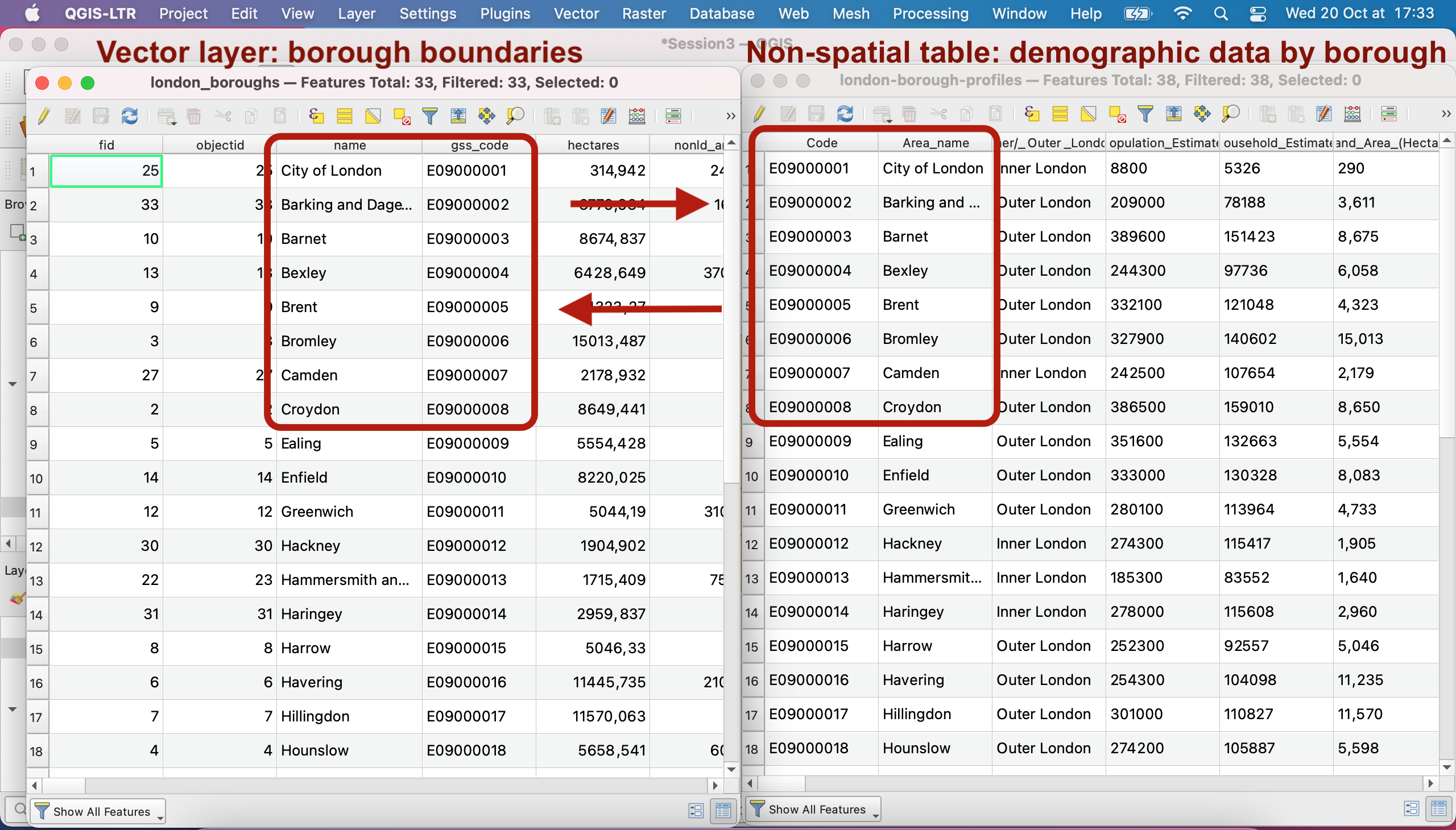
The table contains many fields. Note that the gss_code is a unique identifier; each borrow has a unique code in the format E90000xx. This is an important one for us because it will allow us to perform an attribute join later.
Note that in the Attribute table toolbar, you have access to selecion tools that are also present in your main interface toolbar. You can for instance inverse your selection.
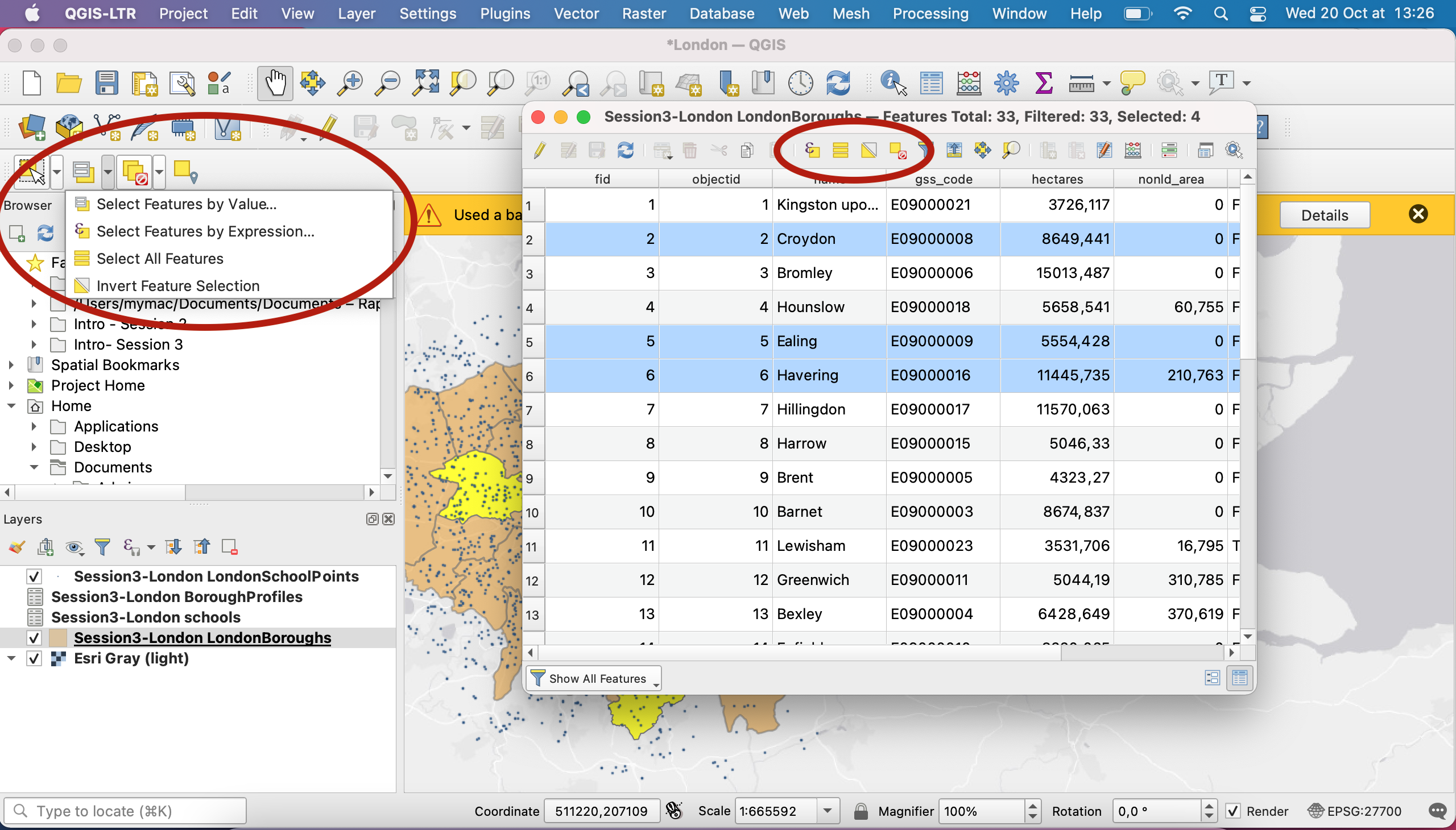
To learn more about the selection tool, read up the documentation page on the various tools available.
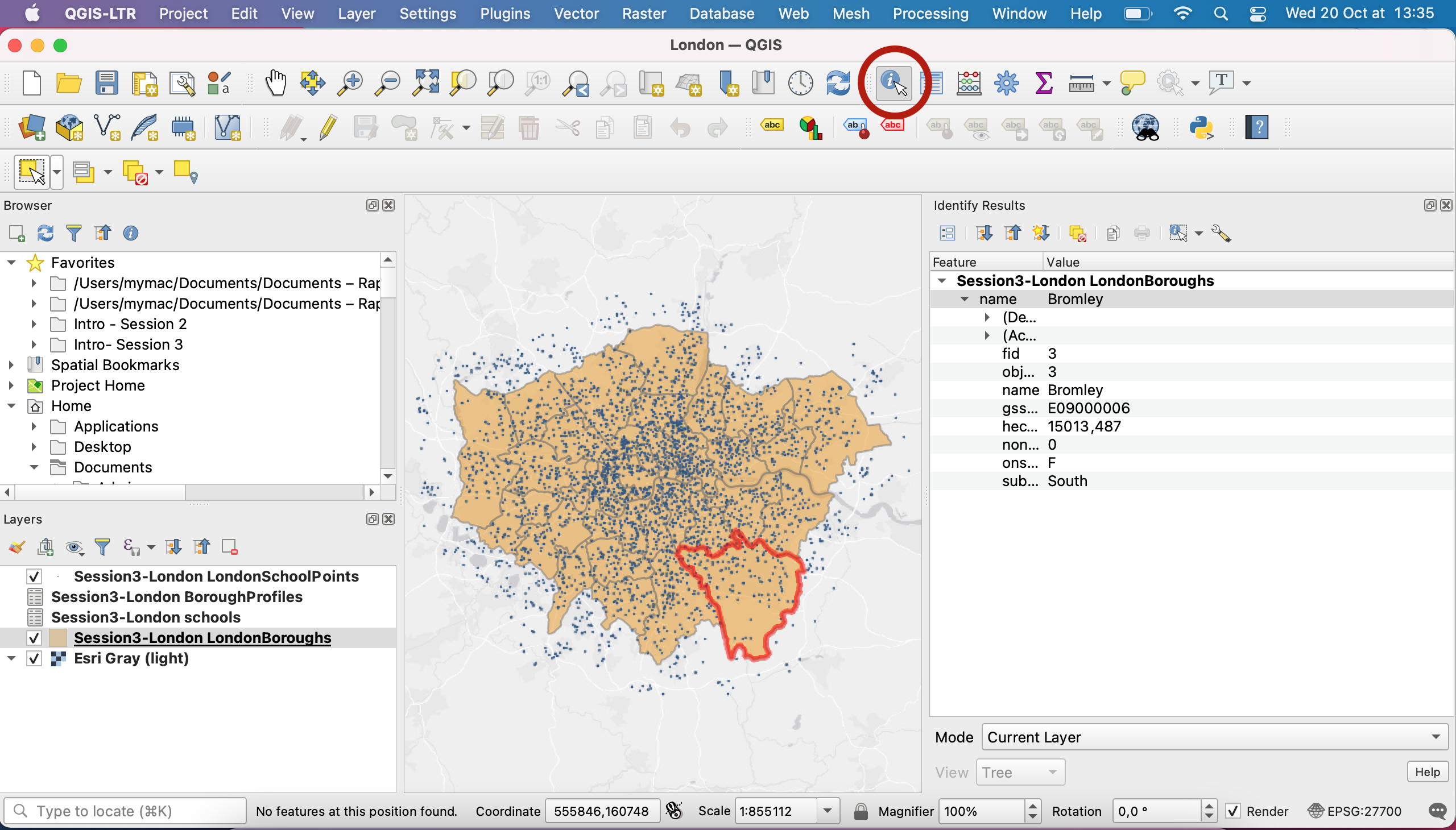
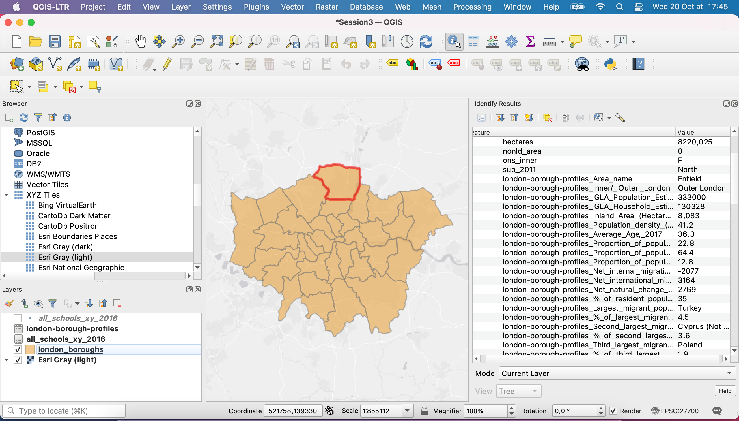
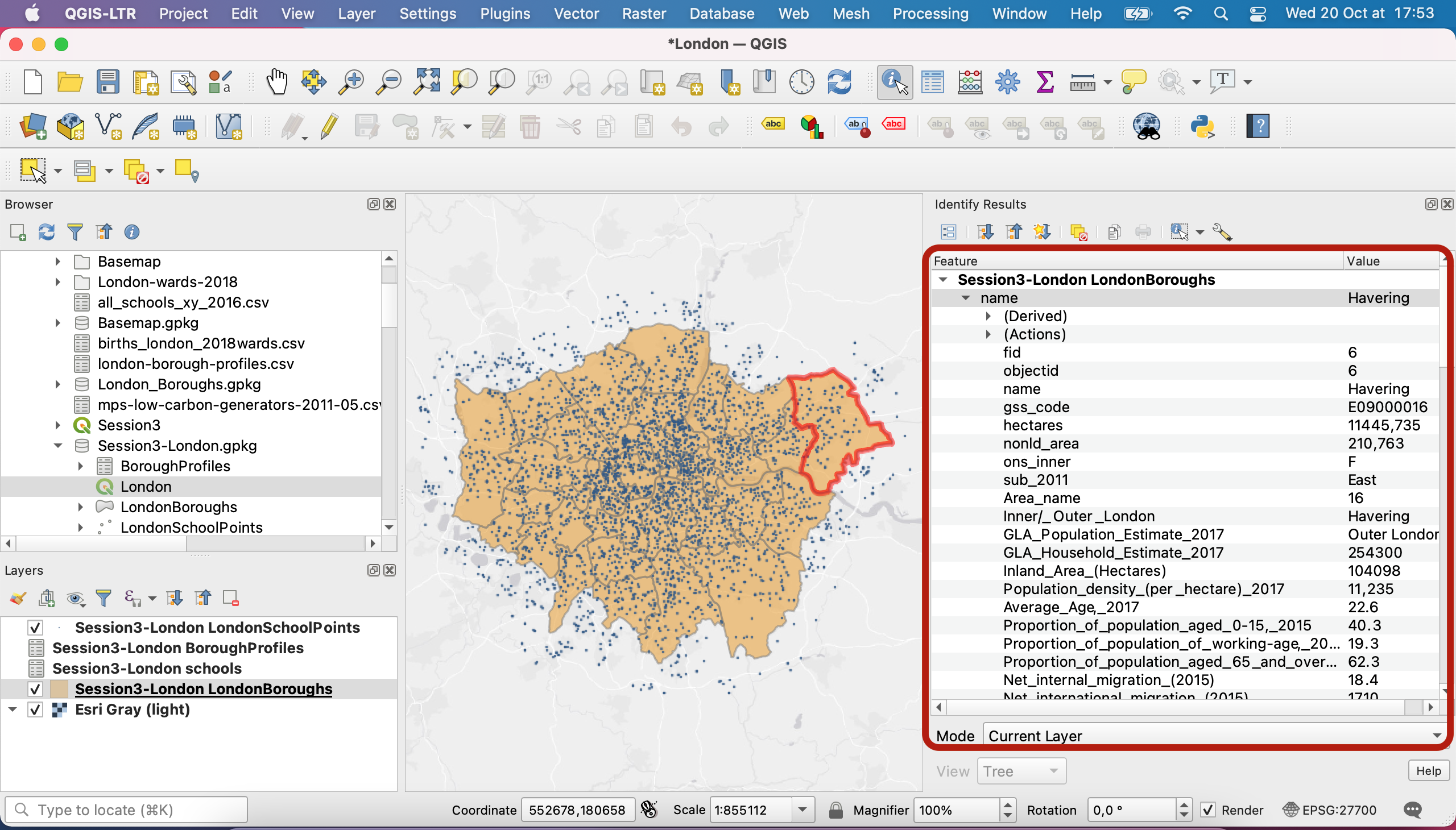
The “Identify features” tool
As seen in the lecture, you can also use the Identify tool to click on features and retrieve the record linked to that feature. Make sure you have selected the layer you are interested in in your Layers panel.
VI. Create a point layer from a *.csv file
In this section, we will import a csv file that contains two fields of interest for us: a longitude and a latitude or x and y. Please note that an Eastings and Northings set of fields would be equally useful.
In QGIS, you can load spatial and non-spatial tables. Vector layers are spatial tables; each vector layer contains a geometry and an attribute table. But you can also load delimited text files in your QGIS projects (files such as *.csv, *.txt, *.dat or *.wkt). They may only contain text, or they may contain coordinates / geometries that you could want to utilize.
If geometry is present in the csv
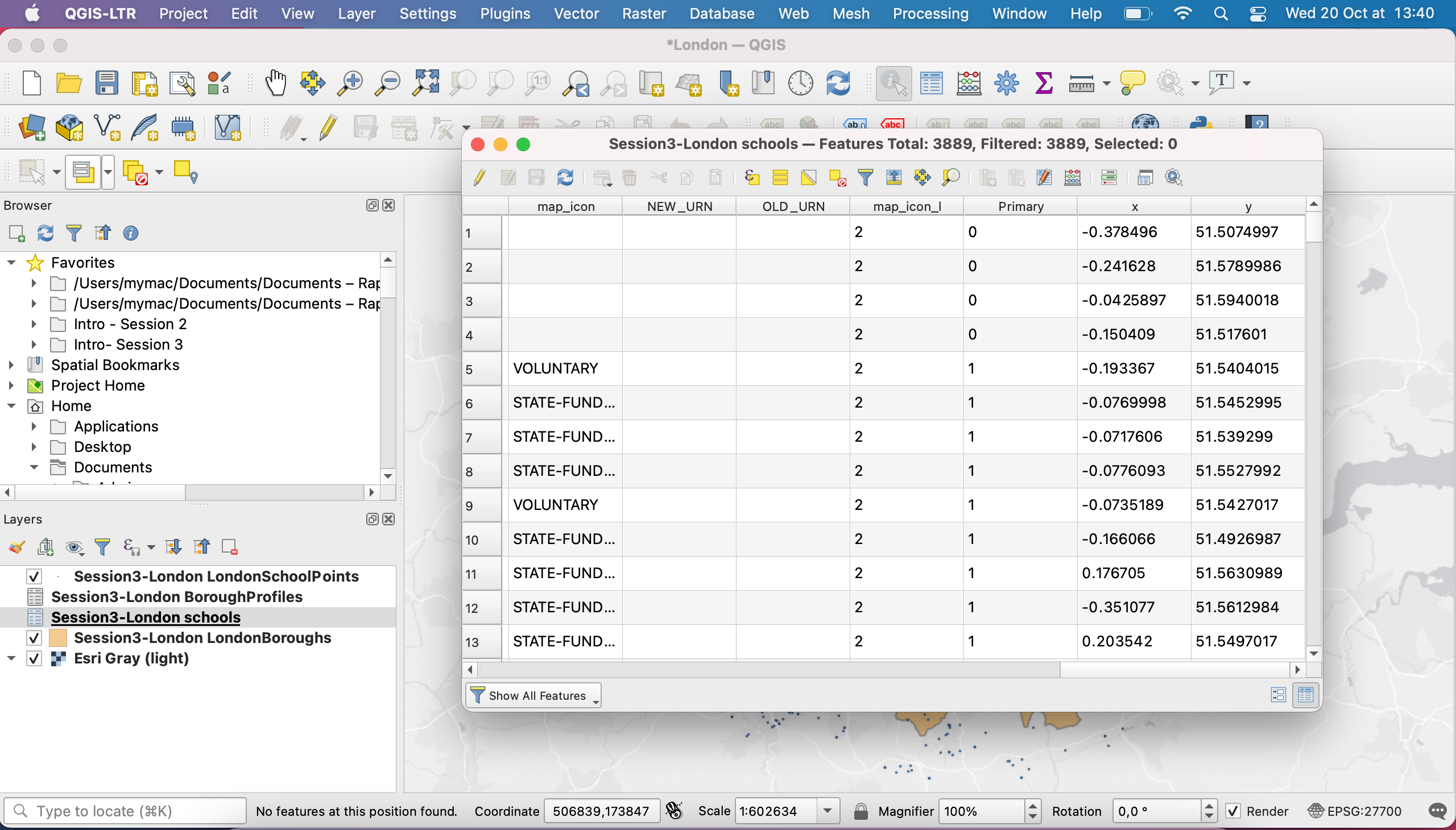
In your geopackage you have a schools layer that contains coordinate fields. It is already loaded in our project as a simple table. As you can see, you can easily access the attribute table of this layer but there is no geometry attached. That’s why in the Layers panel the icon is a table and you don’t have the option to tick or untick that layer; it can’t be added to teh map canvas anyway.
Let’s turn it into a point layer (the final result will be that LondonSchoolPoints layer that is present in the geopackage; as you can see the icon for that layer indicates that it is a point vector layer).
Go back to the GitHub repository and download the file schools.csv into your Session3 folder. Back in QGIS, in your top menu, navigate to Layer > Add layer > Add Delimited Text Layer....
Use the three dots to navigate to the schools.csv file location, and fill the parameters as in the screenshot below. Notice that QGIS has automatically detected the presence of Eastings and Northings fields and used them to populate the geometry fields. Be careful, this time we are working in the British National Grid - CRS (EPSG 27700)!
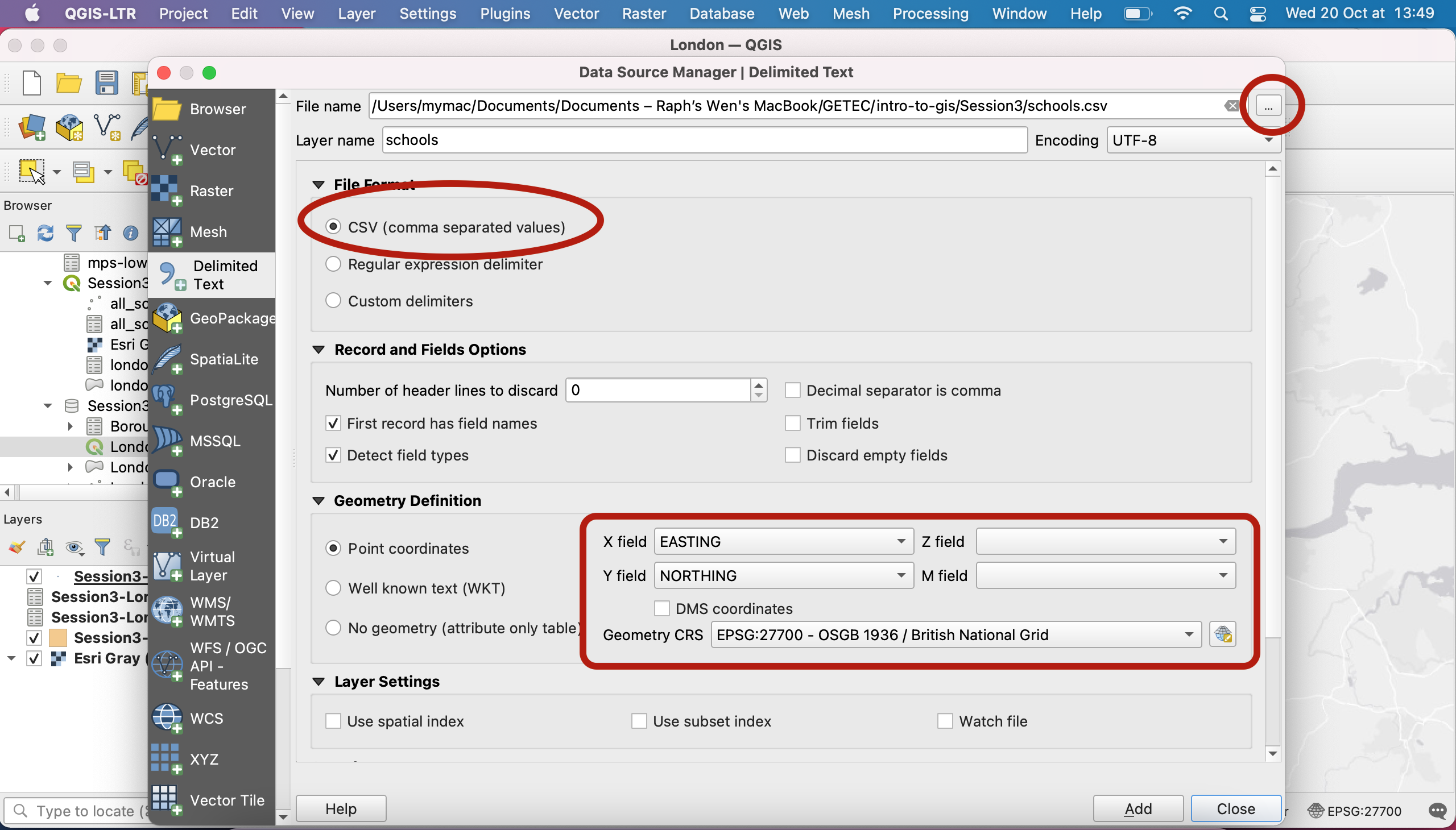
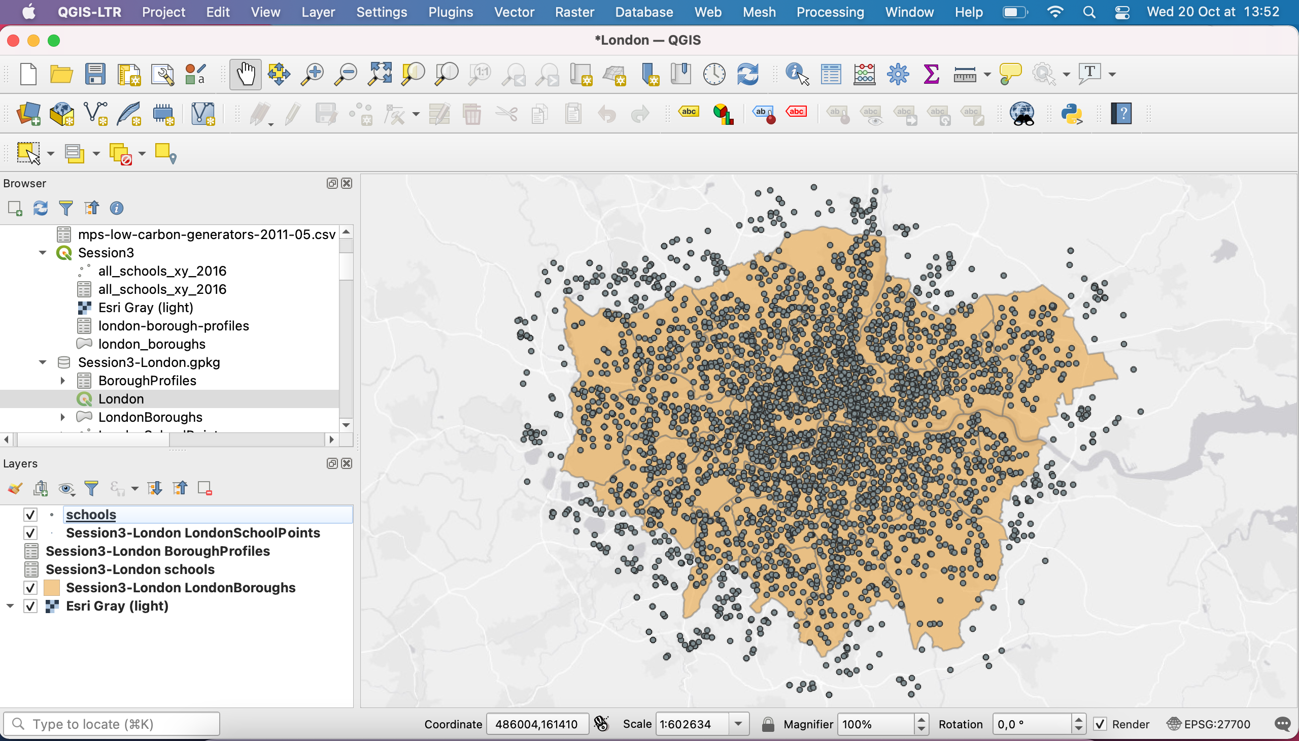
Click Add and close. You now have a point layer where each point is a school!
If you open the attribute table of that point layer, you will find the same information and the same number of rows as in the initial table.
If your non-spatial table doesn’t contain geometry
If your non-spatial table does not contain geometry, then there are 2 options:
- One of the fields is a unique ID that you can join to an existing geometry layer: see next section.
- There is no field that you can in any way link to an existing geometry or location. There is nothing you can do and you can’t use this data in your QGIS project.
VII. Create a table join
A second non-spatial table is available in your geopackage; the BoroughProfiles table. I initially downloaded it as a csv file and it only contains tabular data. If you open the attribute table of this layer, you won’t find any latitude/longitude or eastings/northings fields. However, you will notice the presence of a Code field. It turns out that this code is the same as the gss_code present in the LondonBoroughs polygon layer. When working on census data, national statistics offices will produce boundary files (vector layers) of each census unit, and will make sure to include a column with a unique ID for each polygon. Then, each data table they produce (e.g. on unemployment rates) will also refer to those unique census blocks by referring to this same unique ID in one column.
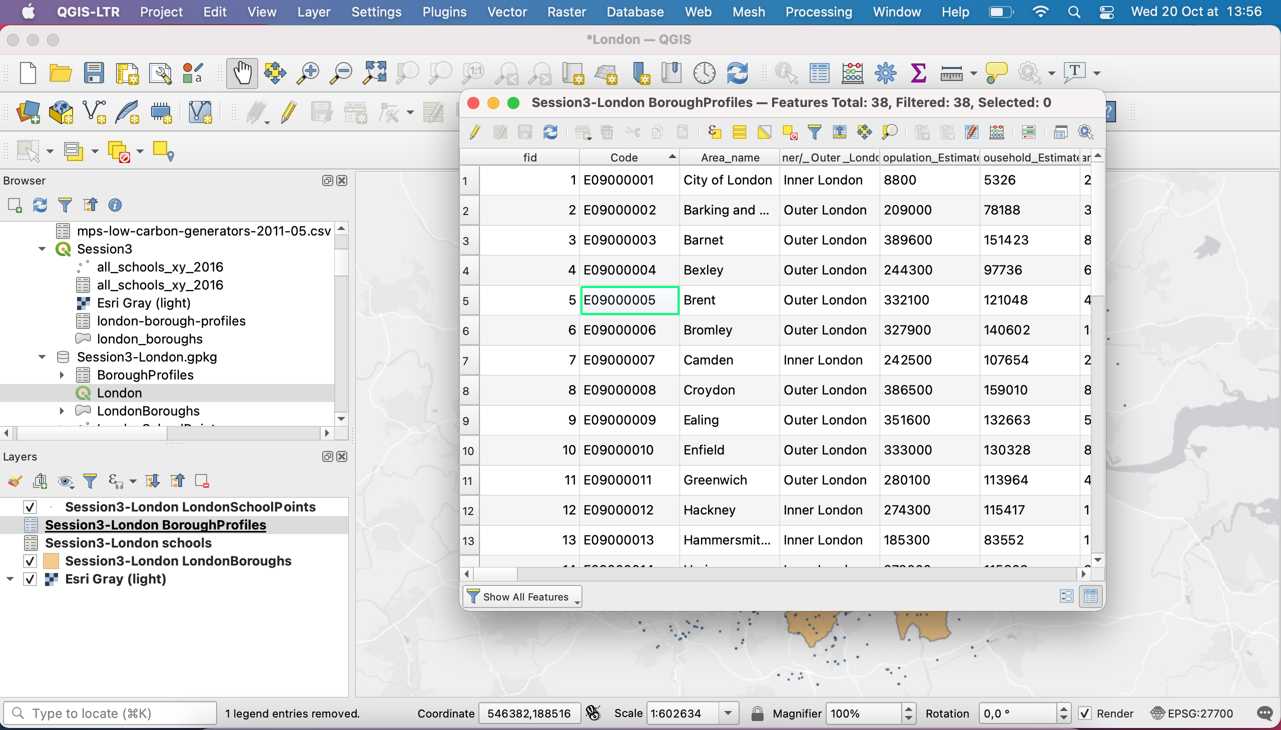
In this case, data is aggregated at the borough level and you have a code to link back each borough polygon with the demographic data that was collected about this borough.
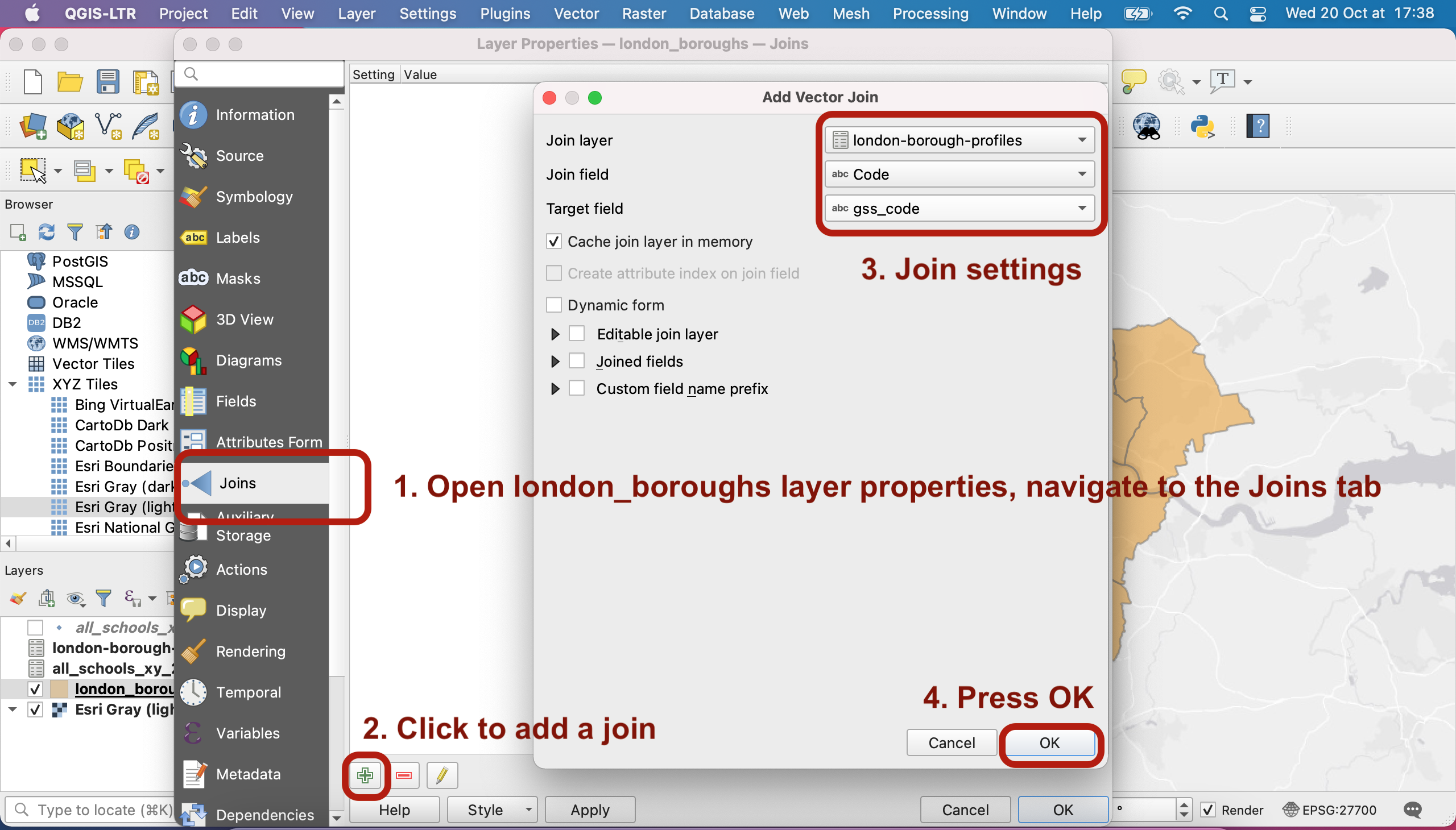
Close the attribute tables. Double-click your LondonBoroughs polygon layer in the Layers menu to open the Layers properties. Go to the Joins tab. The section is empty; click on the green + sign to add a new table join.
The table you want to join is the london-borough-profile table and you want to join using the column gss_code from your polygon layer and the Code from your non-spatial table. Press OK, then press Apply or OK and close your Properties.
That’s it! If you reopen the attribute table, you now have many more fields available about each borrow! Using the Identify features tool you can now get much more information about each individual borough.
Actually, it is really difficult to read these extra information as they all start with a london-borough-profile prefix. You can fix that! Go back to the Joins tab in your London Boroughs layer properties. Double click the join you’ve just created.
Now tick the Custom field name prefix and replace it by something shorter or even nothing at all.
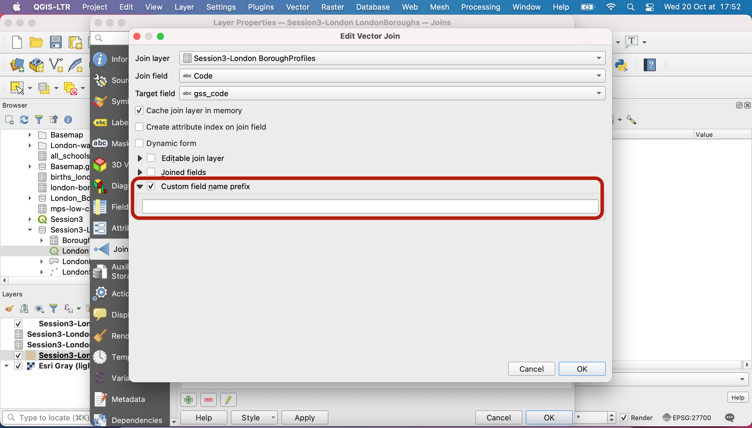
Save and exit - problem solved!
VIII. Create a query to select features based on their attributes
Now that you have all this information about your boroughs, let’s query the data. Let’s figure out which boroughs have a rather high proportion of population of working age. Open your attribute table for the LondonBoroughs polygon layer. Click on the Select by expression symbol. The syntax we’re going to use here can be found in many other places in QGIS. When in doubt, refer to the documentation - it’s very thorough!
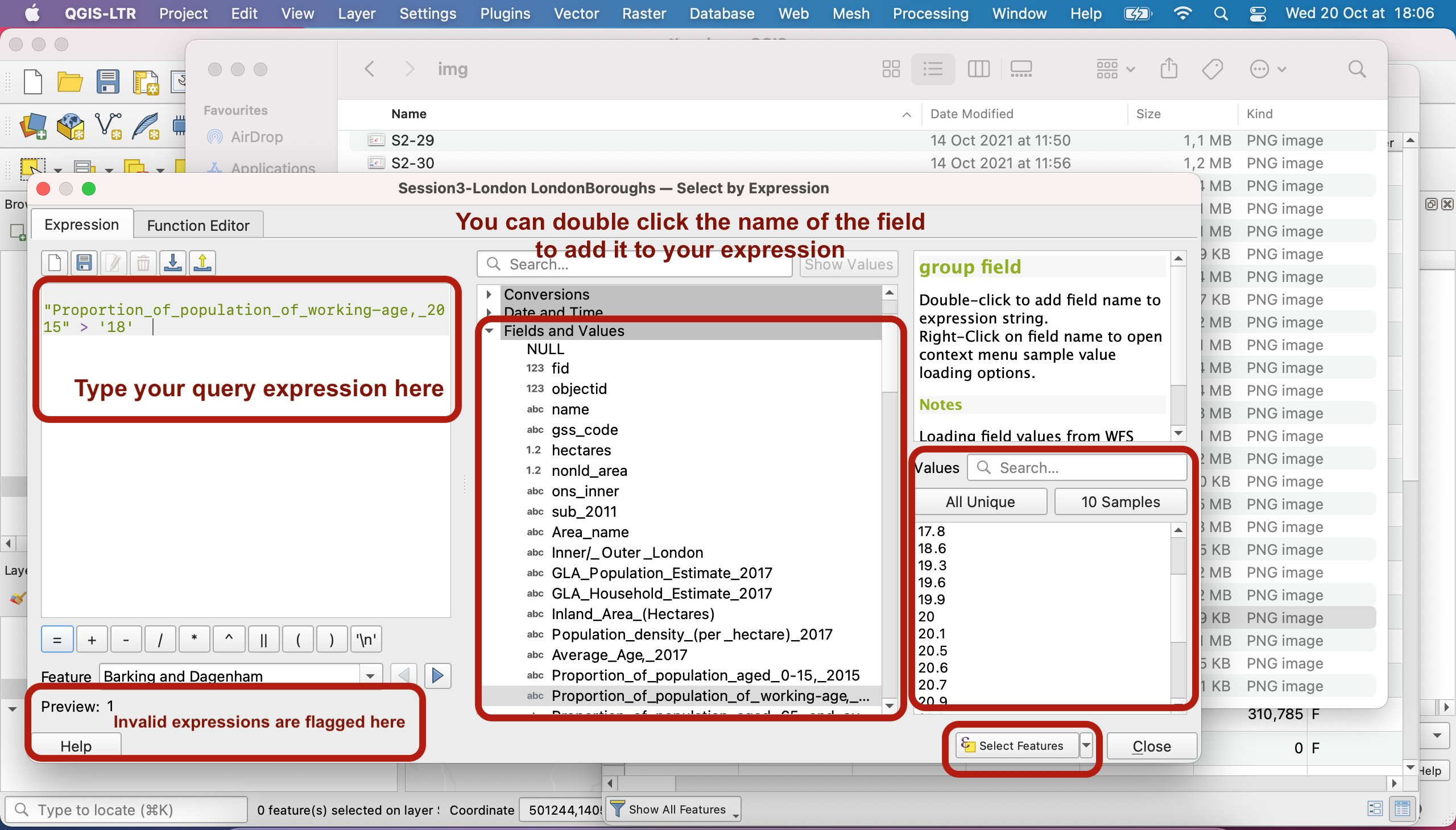
In the left section is the area where you write your expression. At the bottom, it indicates whether you are typing a valid or invalid expression.
In the middle section, you have different families of functions. Click Fields and values to have access to all the fields names from that attribute table. Double click the name of a field to add it to your query expression.
To the right, you can “sample” or see all values from that field to know what kind of values are present in this column. I’m only interested in boroughs where more than 18% of the population is of working age.
IMPORTANT: here, because the field is of type string (you can see a little abc symbol), it looks like QGIS is treating each numerical value like a string. We will see next week how to solve that issue. For now, just type ‘18’ between simple quote marks. Field names use double quote marks and strings single quote marks.
Press Select features and close. You have now selected all the boroughs that match this criteria!
IX. Use queries to only display a subset of your layer’s features
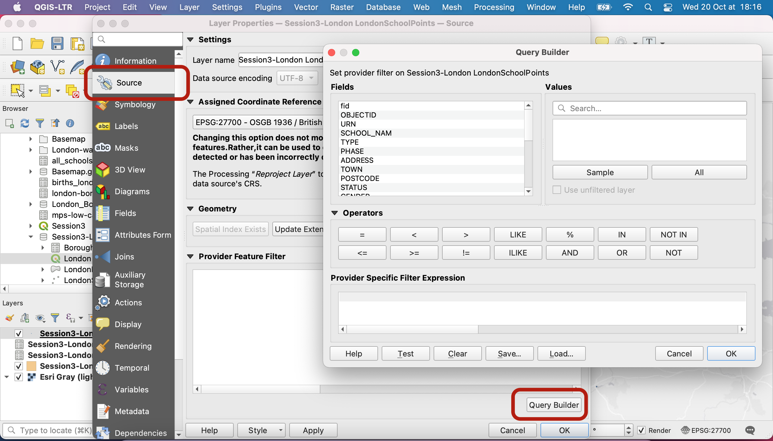
You may use a very similar approach to only display a subset of your dataset’s features, directly from the parameters menu of your layer. This time let’s play with the school point layer. Double click your LondonSchoolPoints layer to open the Layer properties. Navigate to the Source tab. Below the Provider Feature Filter, you should find an empty section. This means no filter is currently applied. Under this white block, click Query builder to create a new filter.
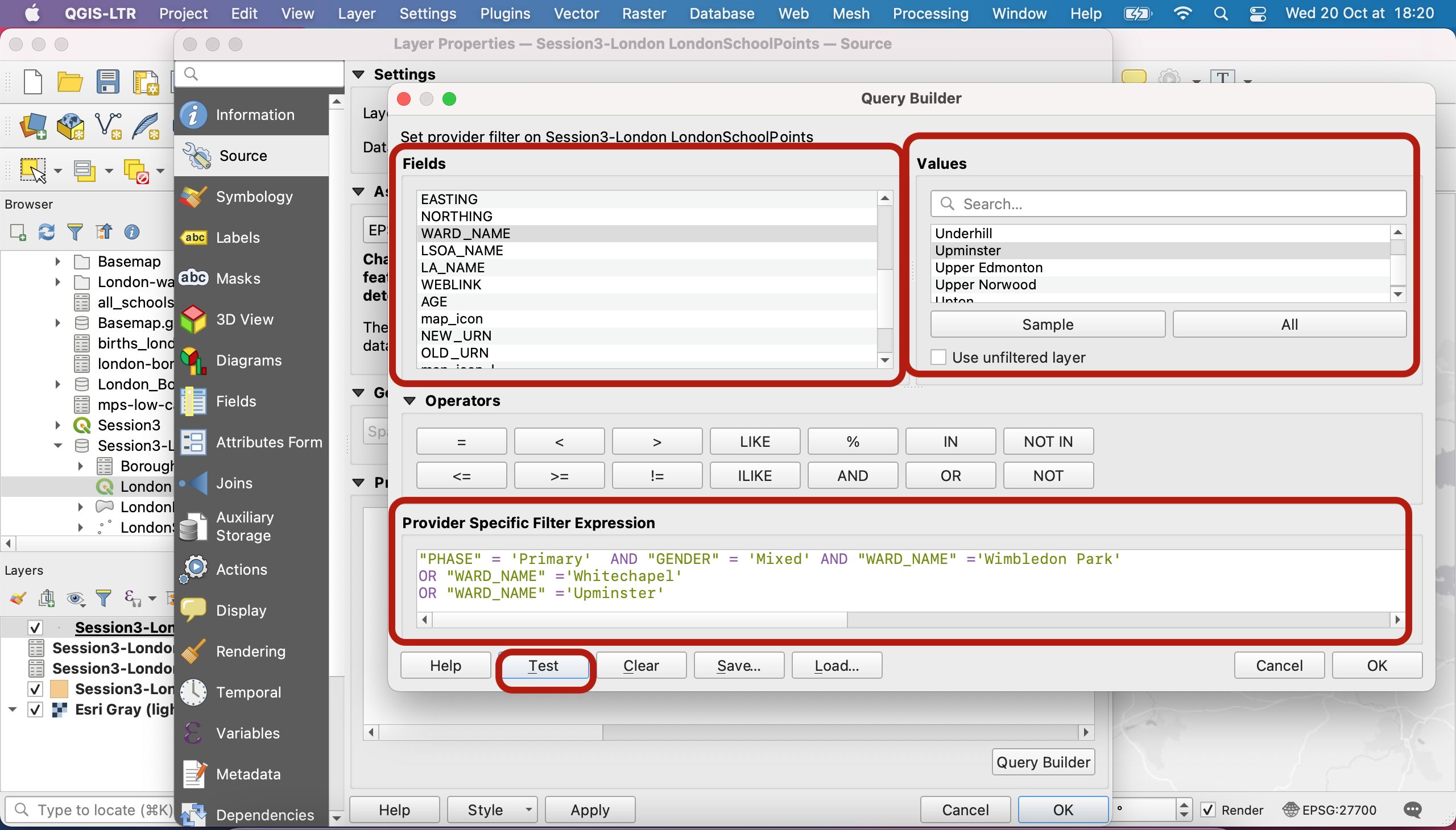
You can for instance write a query (a WHERE clause if we’re using the SQL vocabulary) to find out which mixed-gender primary schools are located in the wards of Wimbledon, Whitechapel or Upminster. Note that, similarly to the Select by expression box from the previous section, you can double-click on field names and the values that you get from sampling the values. You can use the Test button to figure out if your expression is correct and how many features it returns.
Press OK and exit. You can now see that a filter is applied and your layer only contains 28 features. A little filter has also appeared and allows you to directlya ccess and edit your definition query. To remove the filter, erase the expression.
Well done, that’s it for today! Try out the various selection tools and try to build other definition query filters to get more familiar with queries. Next week we’ll look into symbology.