Session 6 - Wrap-up
16 Nov 2021Introduction to GIS · Sciences Po Urban School
Lecturer: Raphaëlle Roffo
I. Session 6 Overview
Download the slides
This final session is designed as a Q&A session. Students should have designed a methodology for the final coursework and are encouraged to prepare specific questions. Students will be able to select topics to be revisited in class, or to hear about more advanced GIS techniques if they wish.
II. Tutorial
Goals:
- Carrying out a flood risk visualisation exercise using vector data symbology and geoprocessing
Context:
In the Greater London Metropolitan Area (GLMA), which local areas are the most likely to get flooded?
What are the demographic characteristics of these areas (age, education, employment status, ethnicity, etc.)? This is an exploratory exercise and not a full analysis.
Data:
Please download all the data in the Session 6 geopackage and unzip it.
Data sources:
- flood_zones: Flood Risk Zones.
- census: Census data for London. It’s a csv file (not geographic) and comes at the LSOA (Lower Super Output area; they are the smallest census unit, like the IRIS zones in France) level…
- … so we also need the LSOA geographic boundaries: the lsoa. And because this LSOA dataset is national…
- … we need the Greater London boundaries, to only keep the LSOAs we need.
III. Joining the census data to the London LSOA boundaries
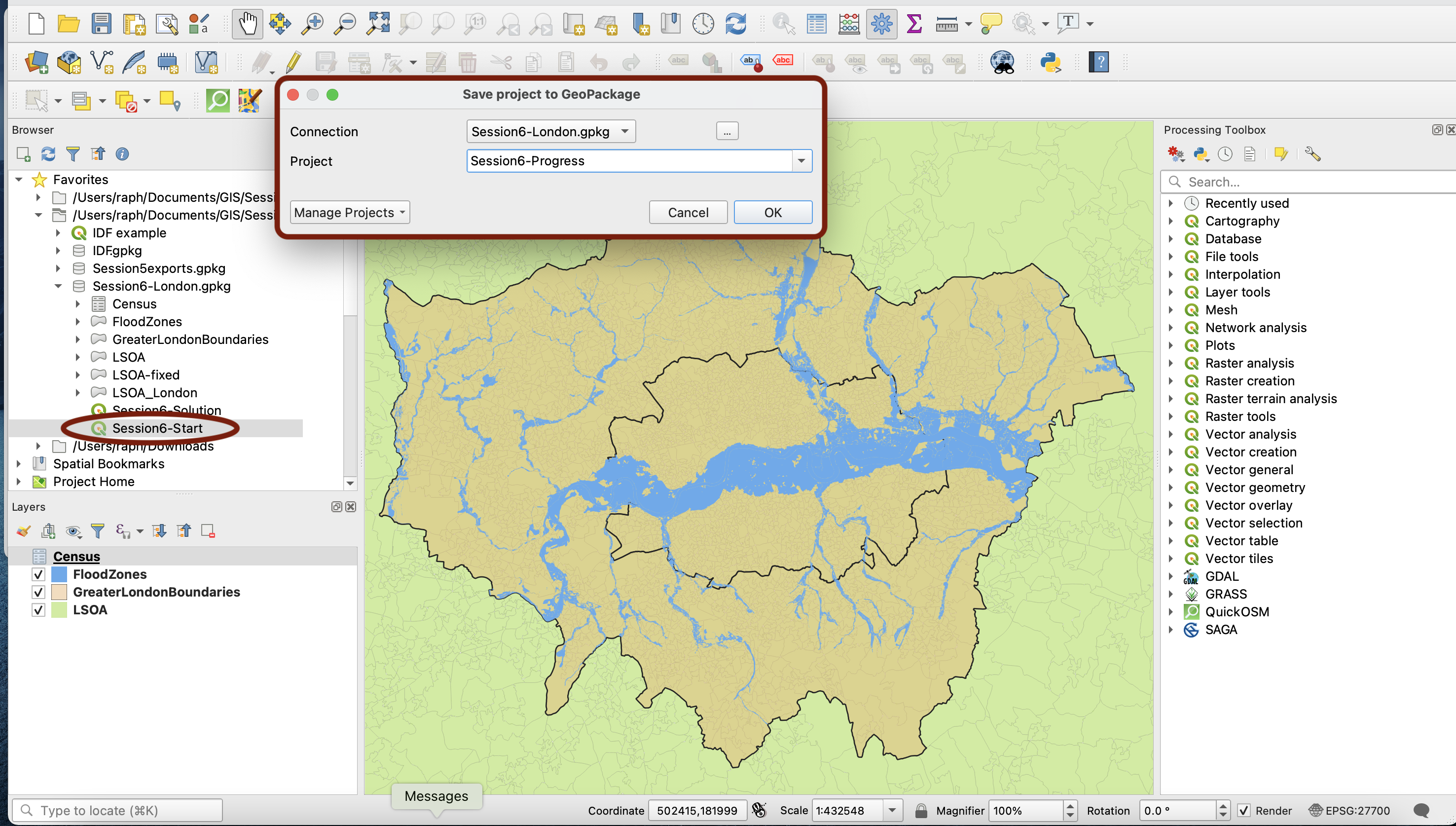
In the geopackage, open the Session6-Start file. Because the LSOA layer is too heavy, I could not add it onto the geopackage. Go download it as a shapefile from the ONS Geoportal.
Now, on your Layers list, you should have the LSOA boundaries, the census table for London at LSOA level, the flood risk zones and the Greater London boundaries. Make sure the CRS is set to EPSG:27700. You can start a new QGIS project to save your progression using your top menu Project > Save to... > Geopackage and in your Session6 geopackage, saving for instance as Session6-Progress. This will allow you to go back to the start if you encounter too many problems, but also to pick up from where you left off if you’re interrupted while doing this tutorial. Remember to save your changes often using the flapdisk icon.
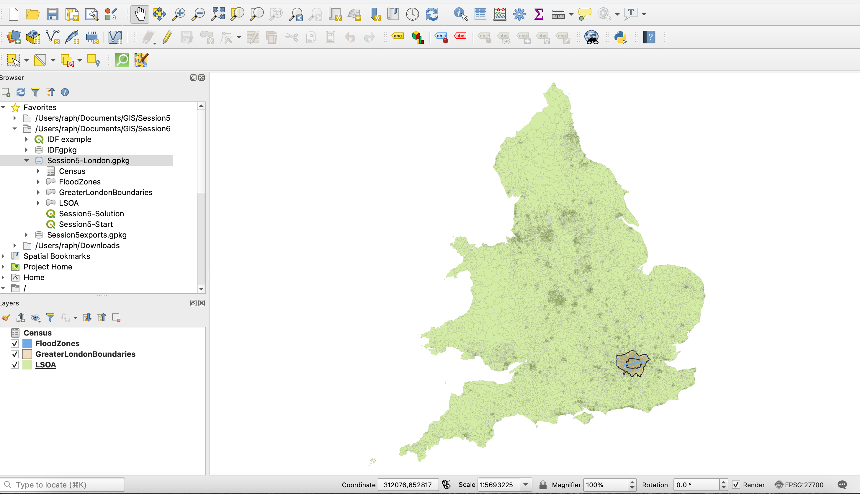
The main thing we want to do with this data is to join the table onto the LSOA boundaries, and to only keep the London boundaries.
But notice that, while we are only interested in the Greater London Metropolitan Area (GLMA) and only have census data for that region, the LSOA file we downloaded covers the whole of England & Wales. If we tried running the join between the LSOA boundaries layer and our census table, it may take a very long time to run due to the large number (34 753!) of features in the boundaries layer (= 34 753 rows in the attribute table).
That’s why in this case and more generally speaking, it can be a good idea to only keep the features of the geographic area you’re interested in before running slightly intensive algorithms such as table joins or geoprocessing. This will speed up the processing time for the following steps.
3.1. Keeping only the Greater London LSOAs: Select/Extract by location
So first, we want to create a subset of the LSOA layer thatonly contains LSOAs in the GLMA.
A first approach to this could be to use the Extract by location tool to create a new layer. To test this, start with Select by Location tool, which will highlight in yellow the polygons that are selected. Extract would directly create a new layer fronm this selection.
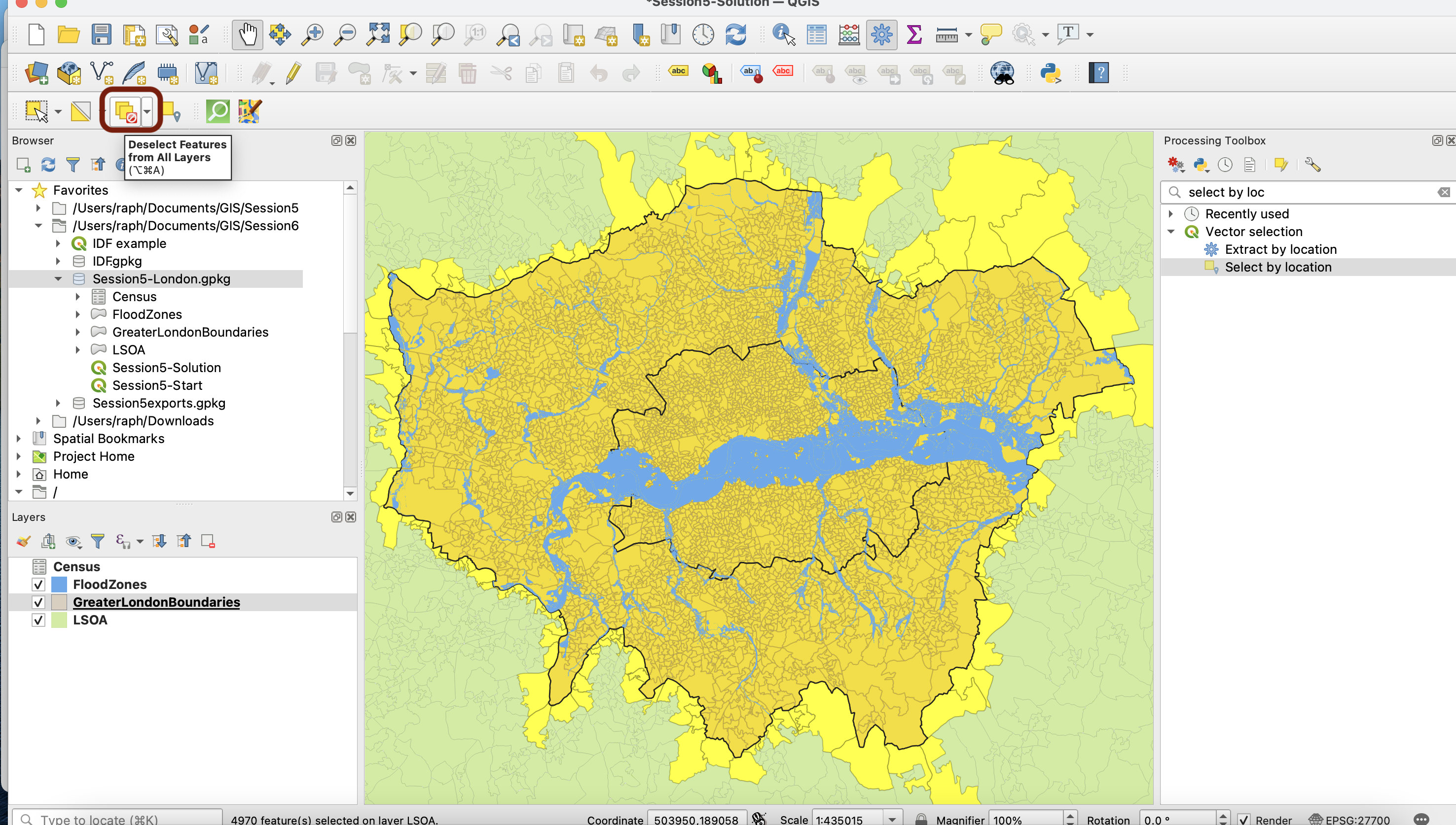
In your Processing toolbox, find Select by location. Try selecting all the polygons from the LSOA layer that are within the GreaterLondonBoundaries:
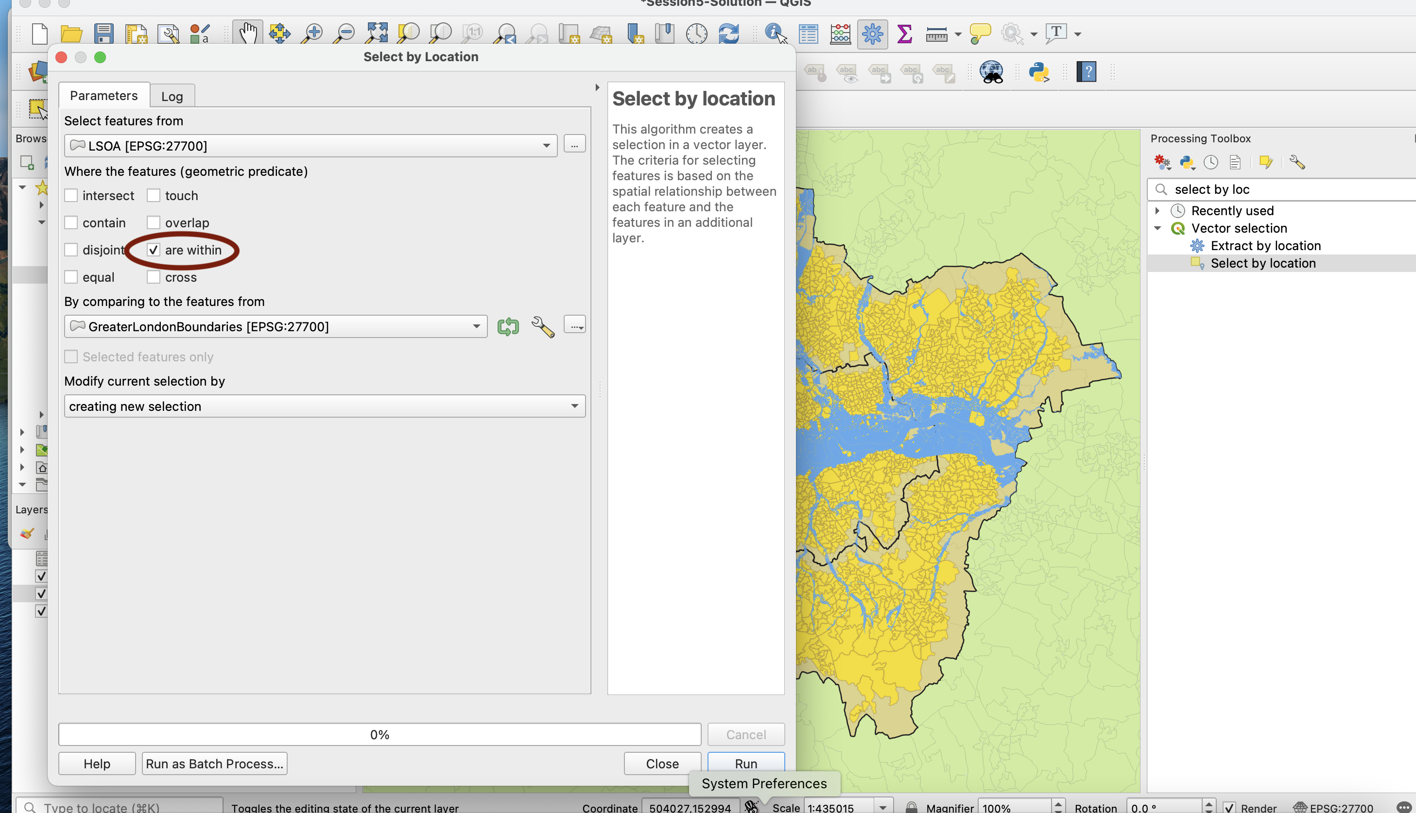
Notice that this is missing out on on the polygons that touch the outer boundary of London.
Now try selecting all the polygons from the LSOA layer that intersect the GreaterLondonBoundaries:
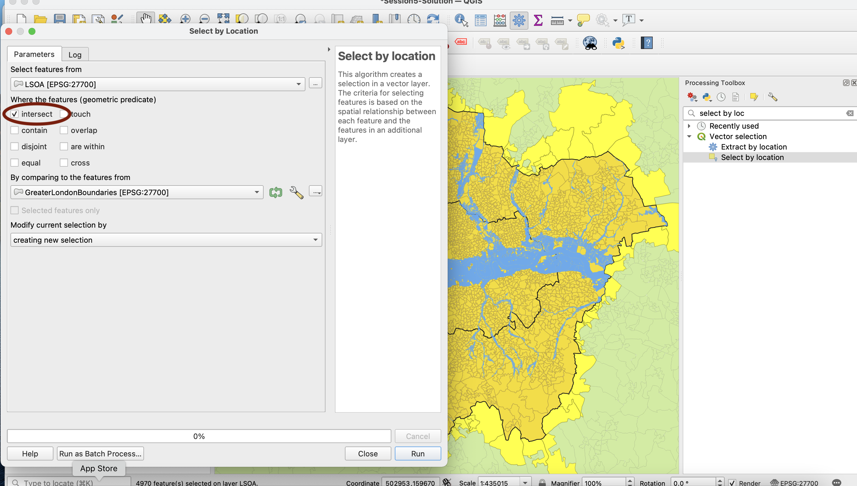
Again, this is not ideal as it’s actually capturing bits of LSOAs that cross the outer boundary of GreaterLondonBoundaries.
You can press this button to clear your selection.
3.2. Clipping & Handling invalid geometries
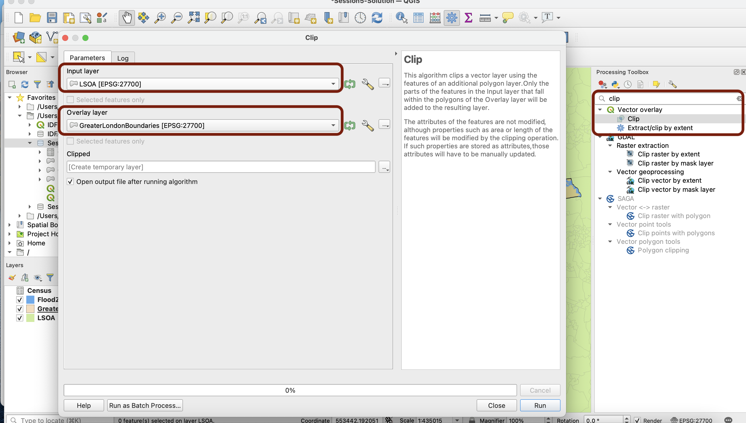
Instead, you want to use the Clip tool to get a neat, cookie-cutter like selection of LSOAs within the GLMA boundaries. Find the Clip in your Processing toolbox and set it up to clip your LSOAs to the shape of GreaterLondonBoundaries.
When you press run, you should get this red error message:
Feature 3173 has invalid geometry”.
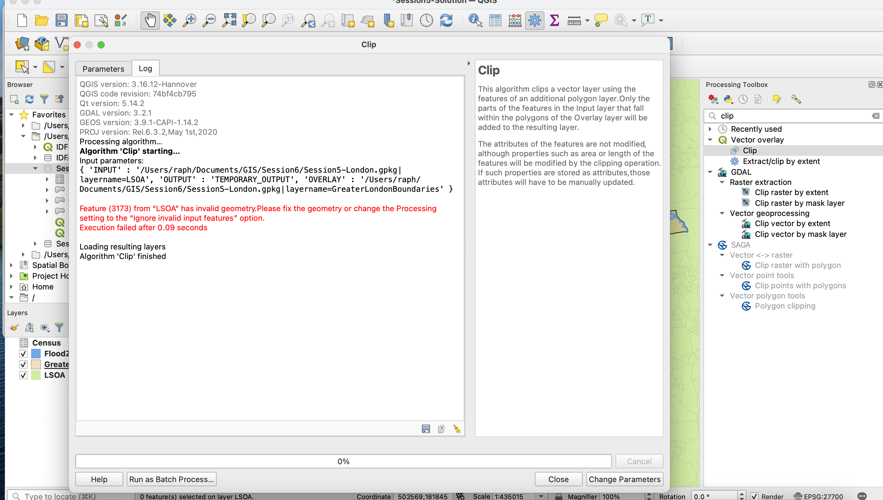
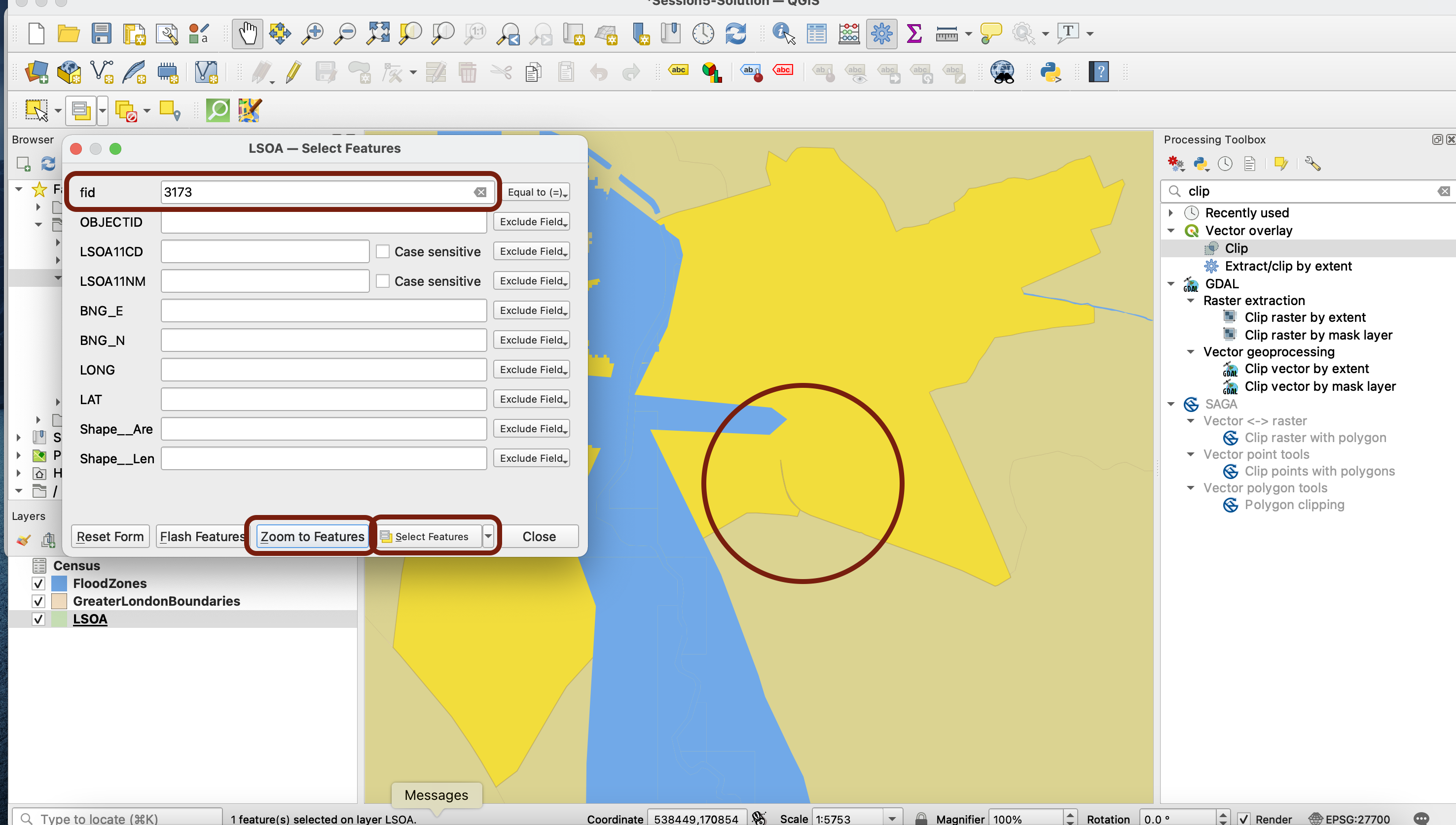
The feature number always refers to the unique identifier of the feature (column OBJECTID or FID in some cases). To look into it, you can use the Select by value or Select by attribute tool from your toolbar (or from your Processing Toolbox panel):
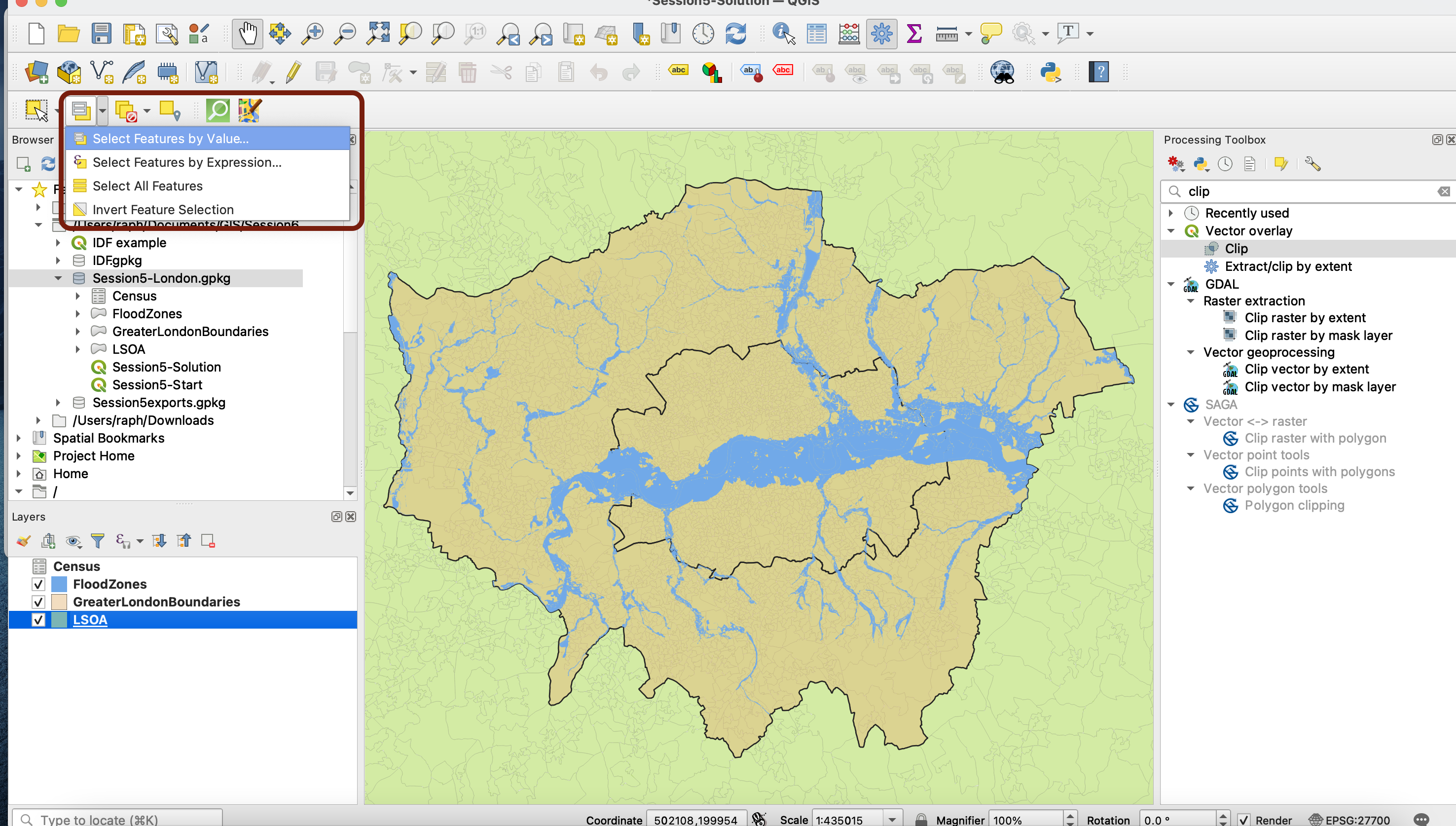
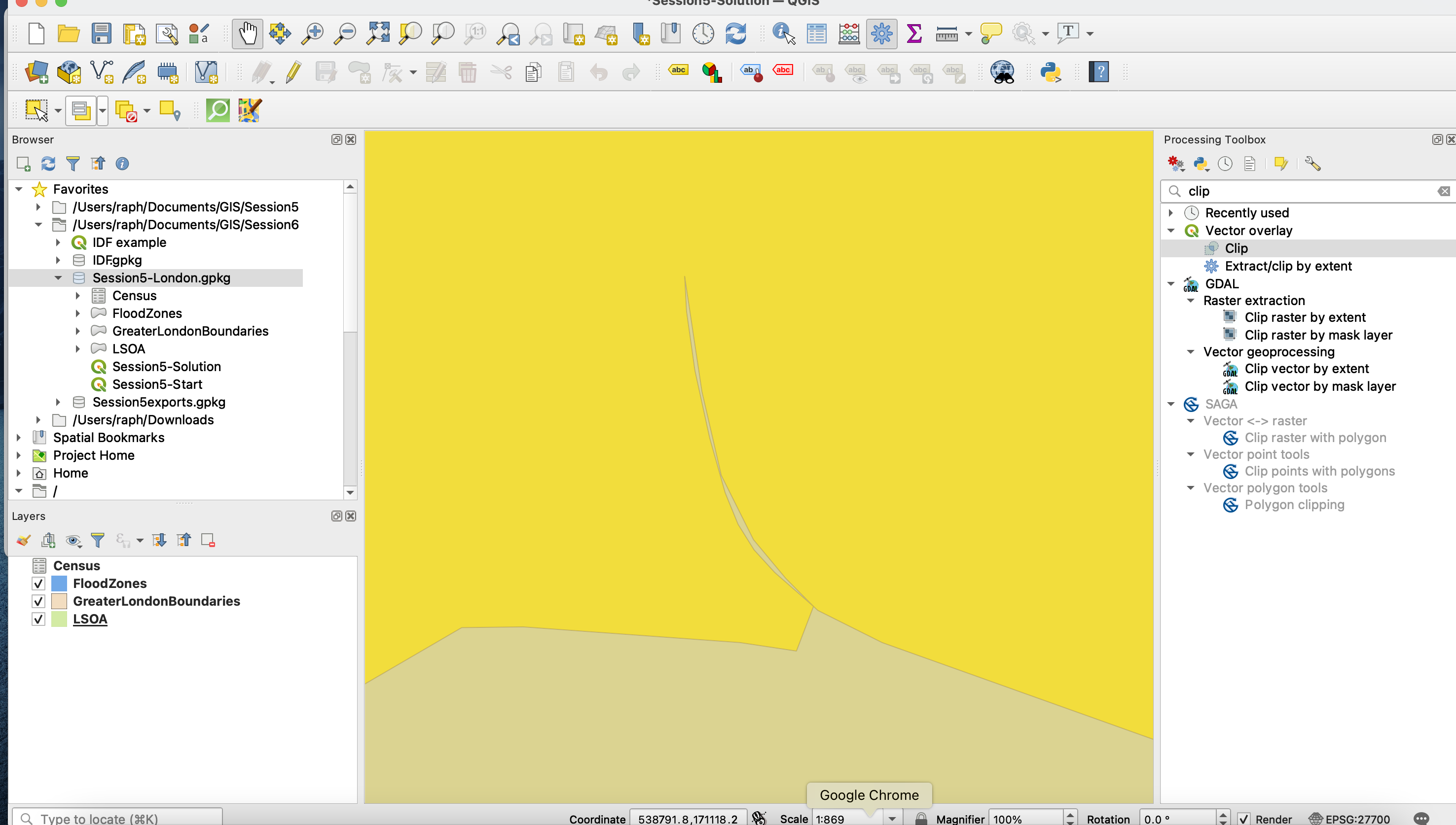
Find the feature in the LSOA layer that has fid=3173, then select it and Zoom to Features. Can you see the odd shape circled in red in the screenshot below? This is an invalid topology where a geometry intersects with itself.
If you zoom even more you’ll see the that the polygon has vertices that cross each other; this is what’s causing the error. Invalid topologies are not uncommon; they are geometries that do not satisfy some fundamental rules about vector geometries. For instance, in a given layer you cannot have two overlapping polygons or geometries that intersect with themselves. When you use a layer with invalid geometries as input into a geoprocessing algorithm, it will fail to run.
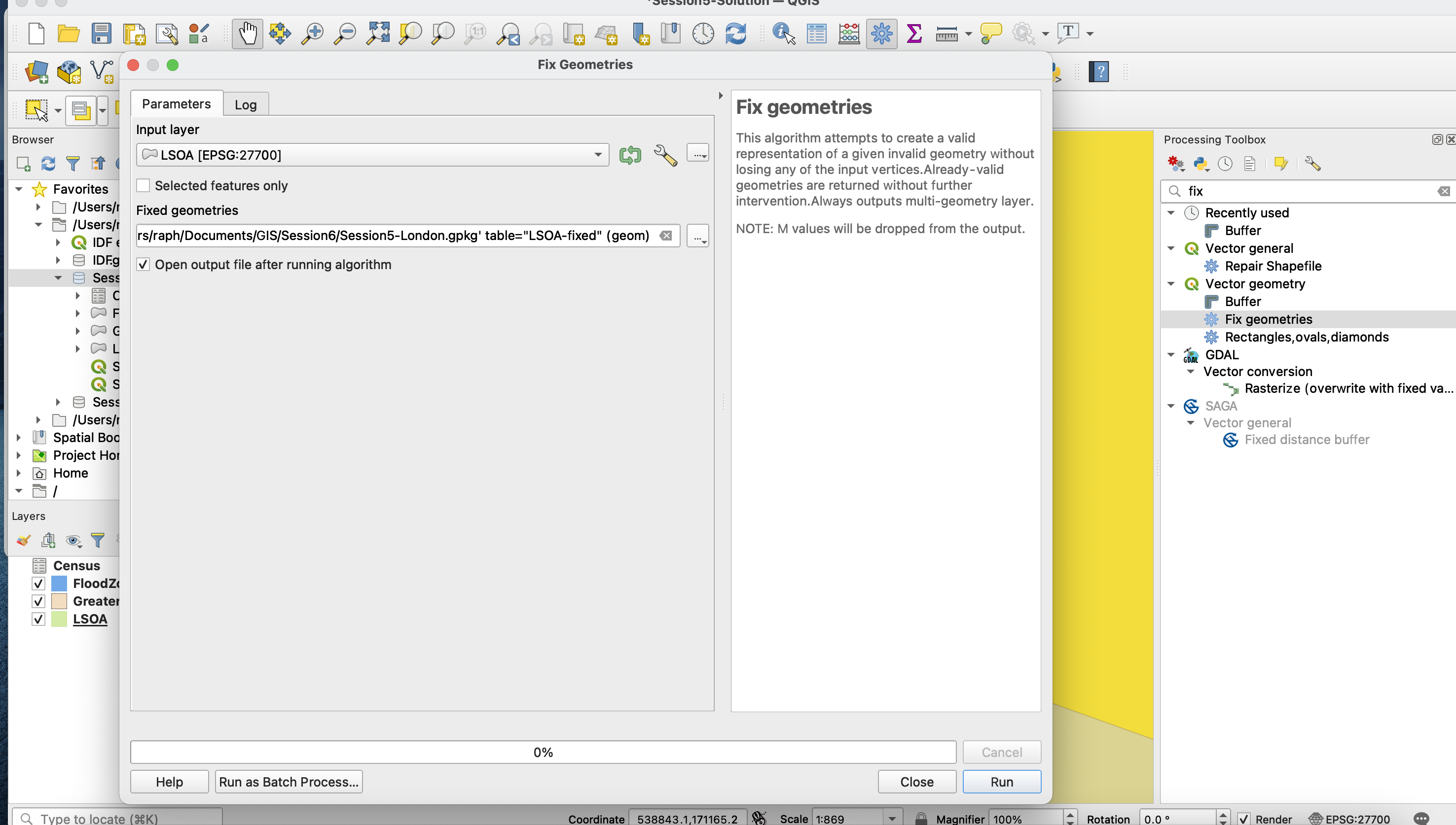
To fix this problem, let’s use the Fix geometries tool. The input is your LSOA layer, and save it directly to your geopackage, with a descriptive name. You can then copy the styles from your LSOA layer into your new, fixed layer before unticking/removing the original LSOA.
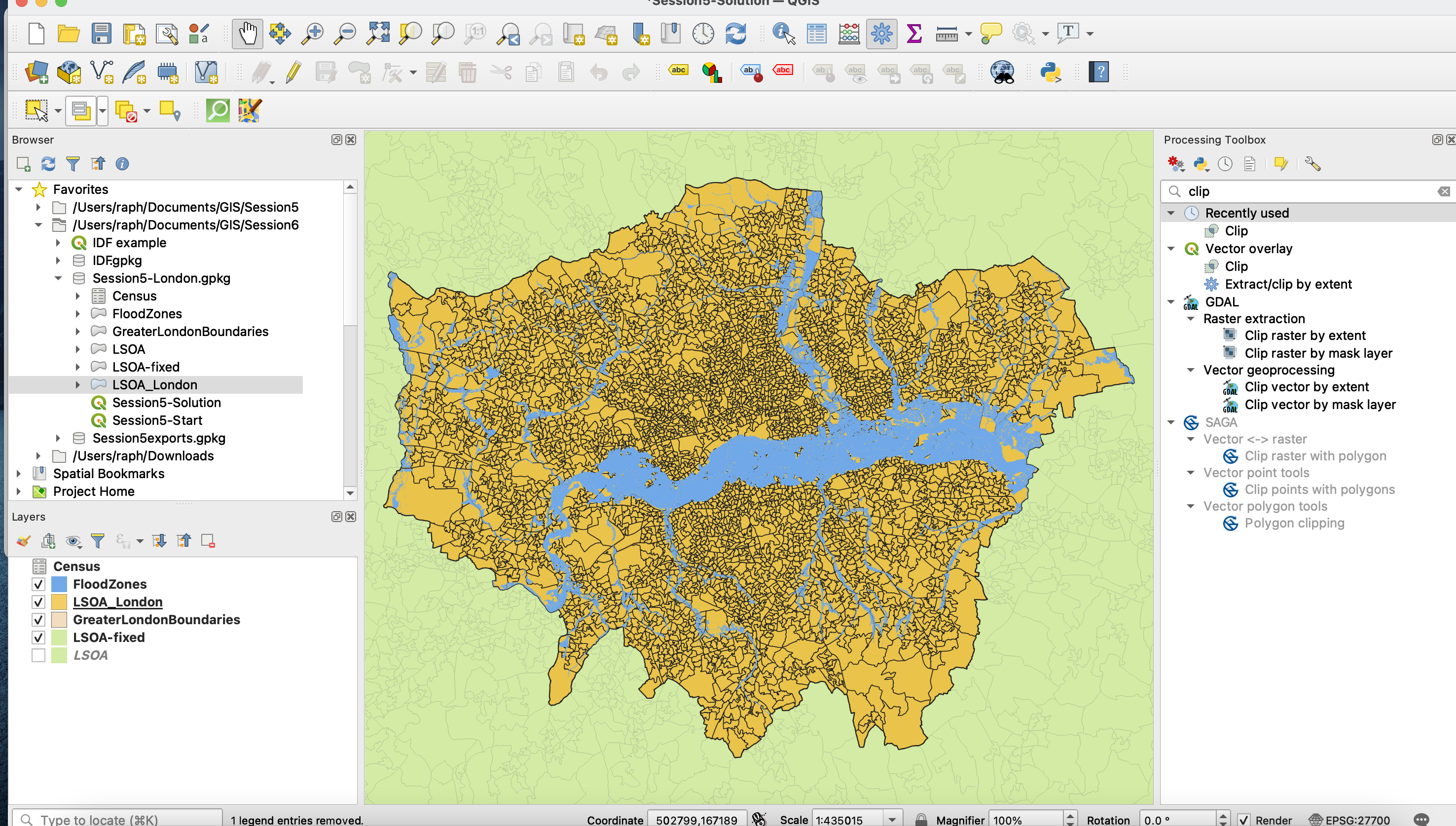
Now, you can run your clip using the fixed layer as input - it should not throw an error this time! Make sure to save it in your geopackage.
3.3. Performing the table join
The census data comes as a non-spatial table. We want to combine information from that table and the geographic boundaries of the LSOAs into a single dataset, using a table join.
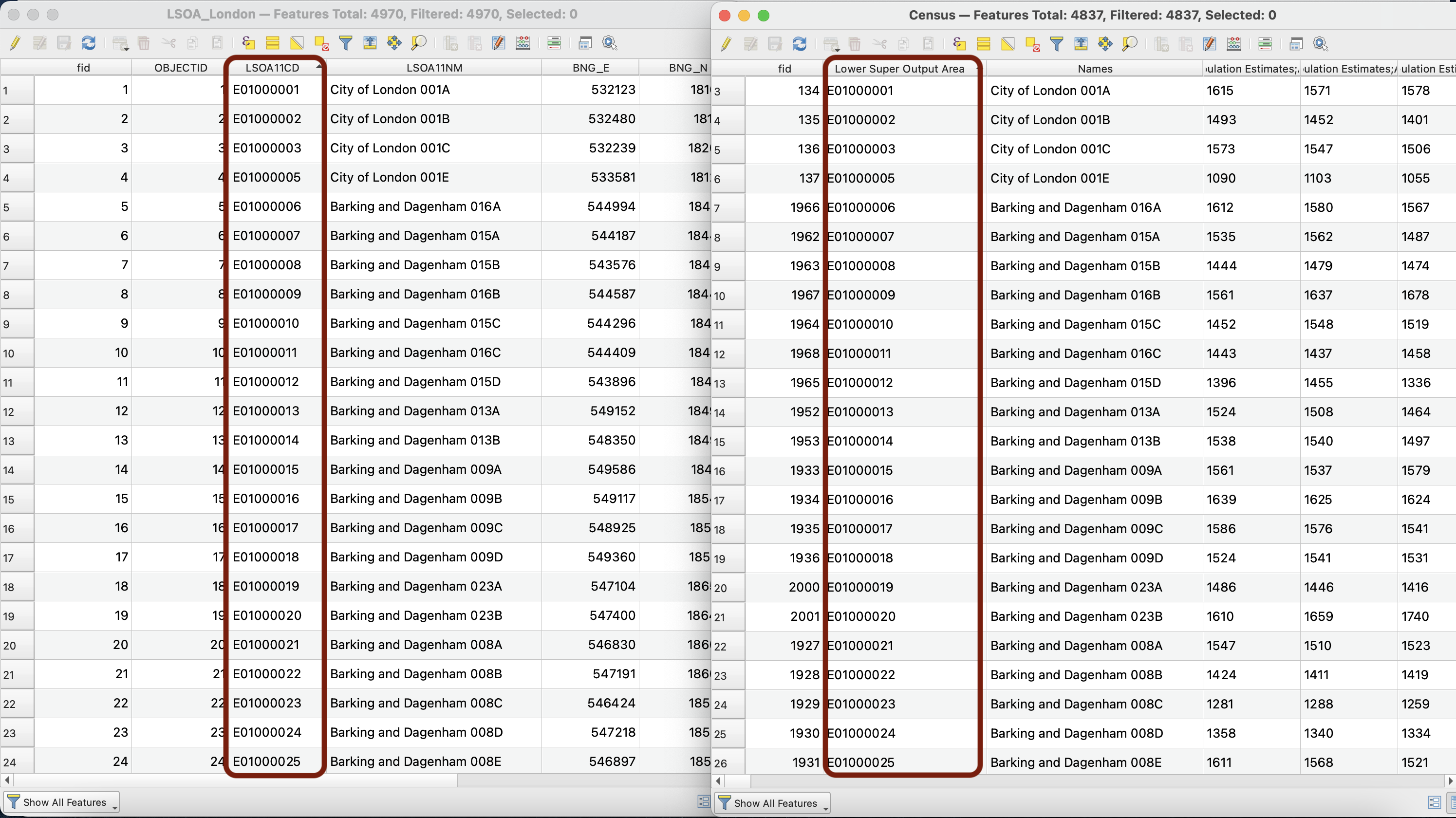
If we look at the attribute table for the London LSOA layer, it contains the LSOAs in Greater London, with some basic information and a column with a unique identifier for each LSOA: the LSOA11CD column.
If we look at the attribute table for the London census table, it contains a lot of variables but also a Lower Super Output Area column which contains very similar codes to LSOA11CD. This is the official LSOA code, produced by the Office for National Statistics (ONS). After a couple quick checks (comparing Names and Codes in both table), we confirm that they are indeed the same codes in both tables.
Note that the LSOA11NM and Names columns would also seem to be good matches as Key fields for the join; however names are more prone to spelling differences (a space or apostrophe might be present in one table and not the other). That’s why when available, you should alwyays opt for the standardised code instead!
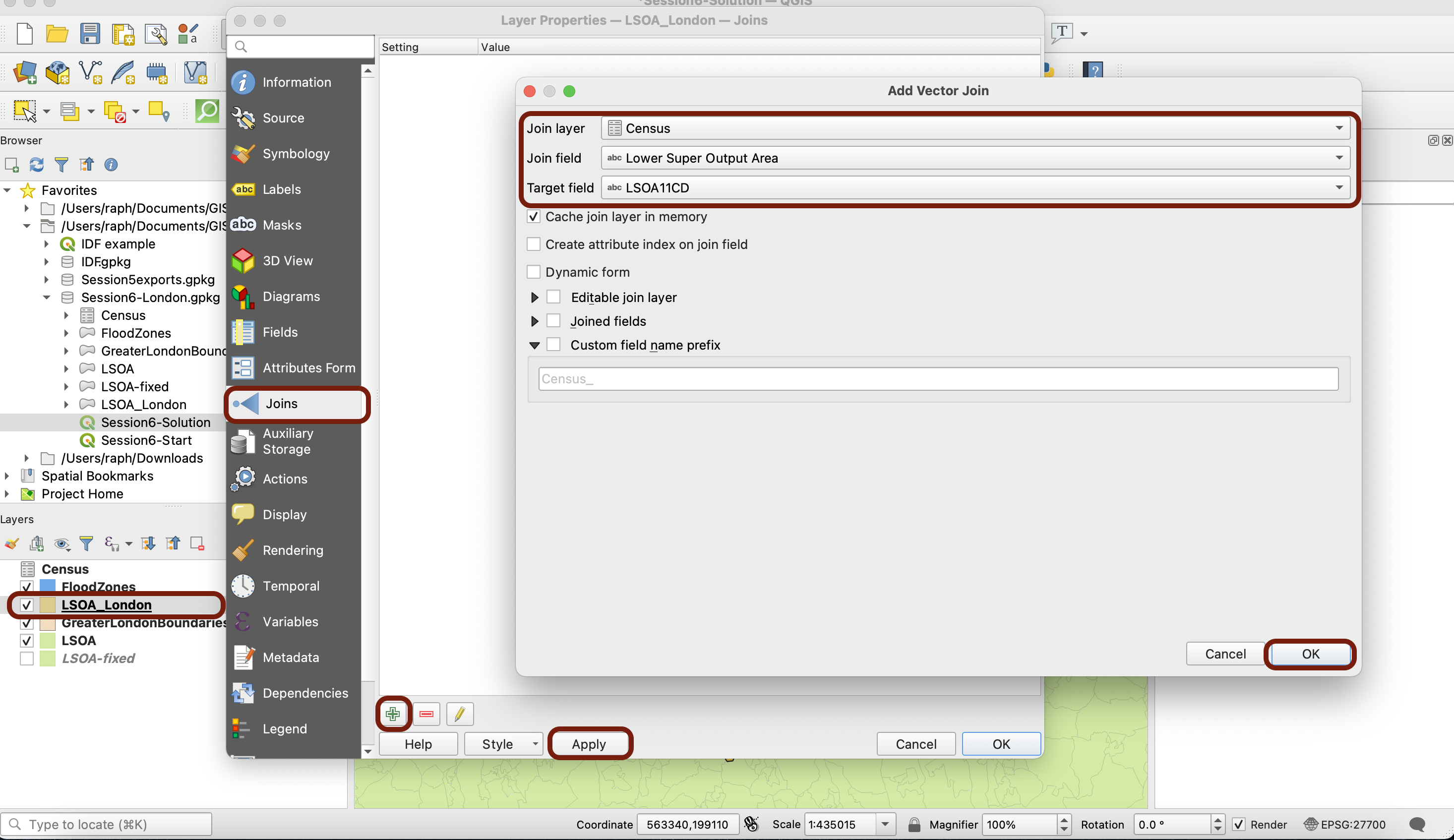
Double-click your London LSOA layer to access the Layers properties, navigate to the Joins tab and click the Green Plus sign to create a new join based on those two fields. Press OK, then Apply.
Now can be a good time to save a copy of this “super” LSOA Census layer in your geopackage. Right-click your London LSOA layer, Export > Save Features as... and give it a descriptive name.
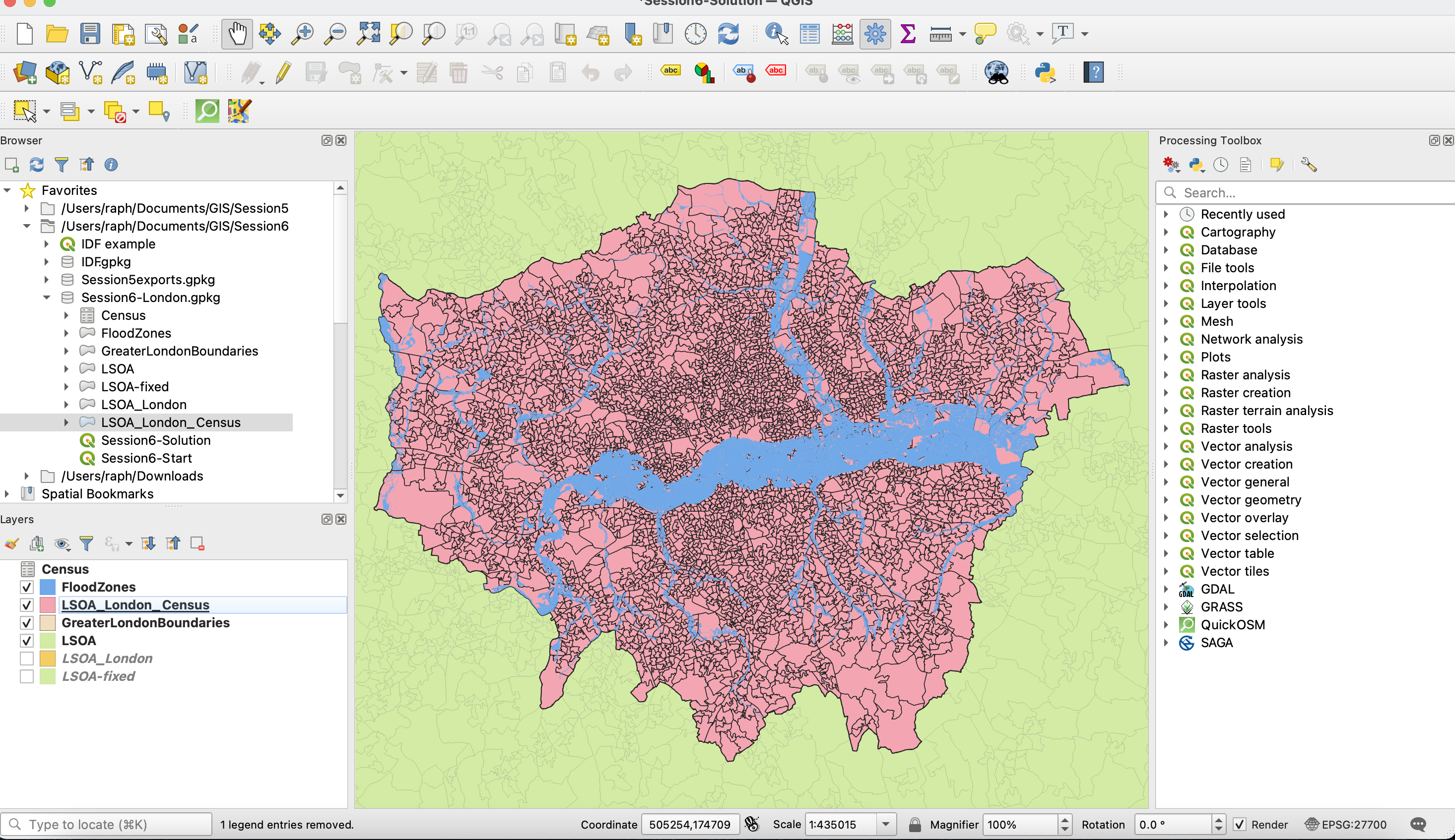
IV. Population density choropleth
4.1. Fixing the data type
Now, among all the variables in the census, we are interested in population density, present in the field Population density; Persons per hectare 2013. We want to build a choropleth of population density, which we will later on combine with flood risks exposure.
The field is not available for the use of graduated symbology. Can you guess why?
If you recall from our previous tutorial, the problem comes from the data type of the field. In your Layer symbology, under the Fields tab, open the field calculator and see if you can figure out which expression you need to write to obtain a numerical PopDensity field.
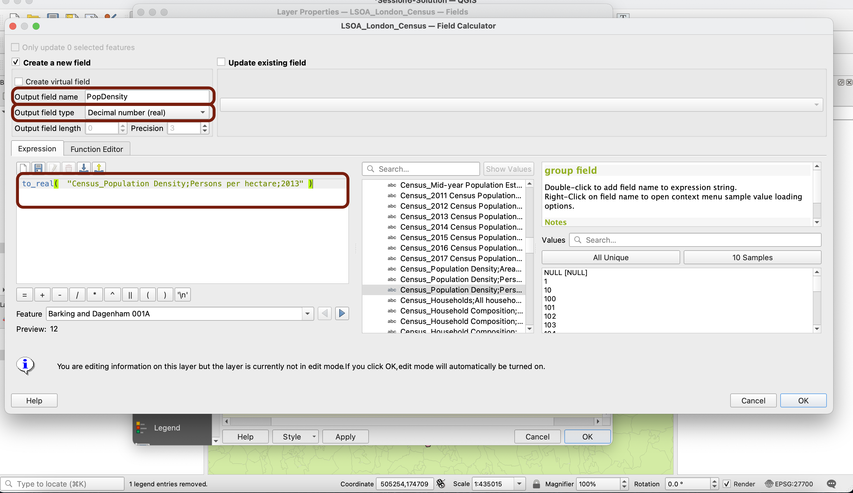
Once your field is created, remember to exit Editing mode by pressing the yellow pencil and saving your changes!
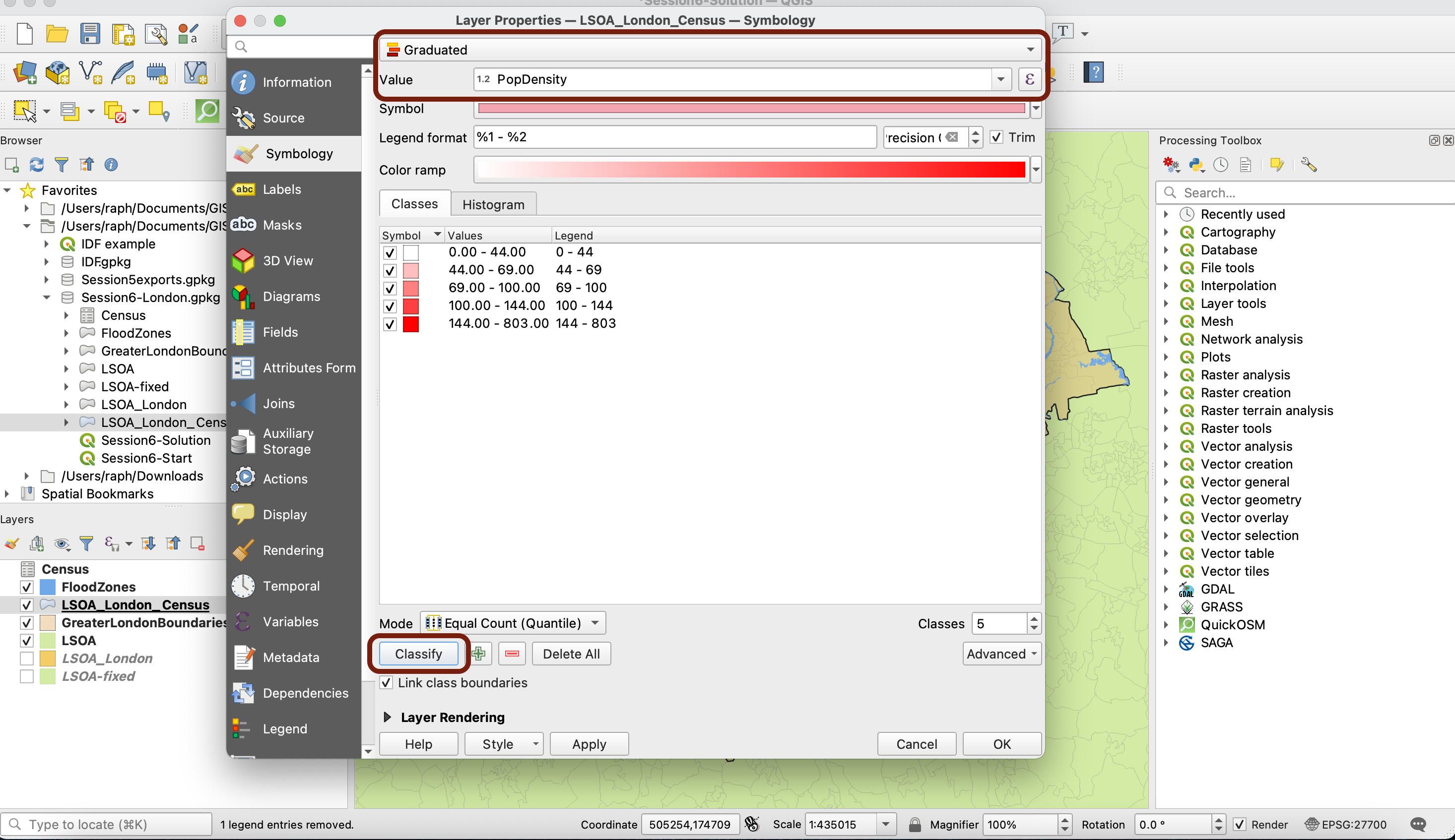
4.2. Symbology
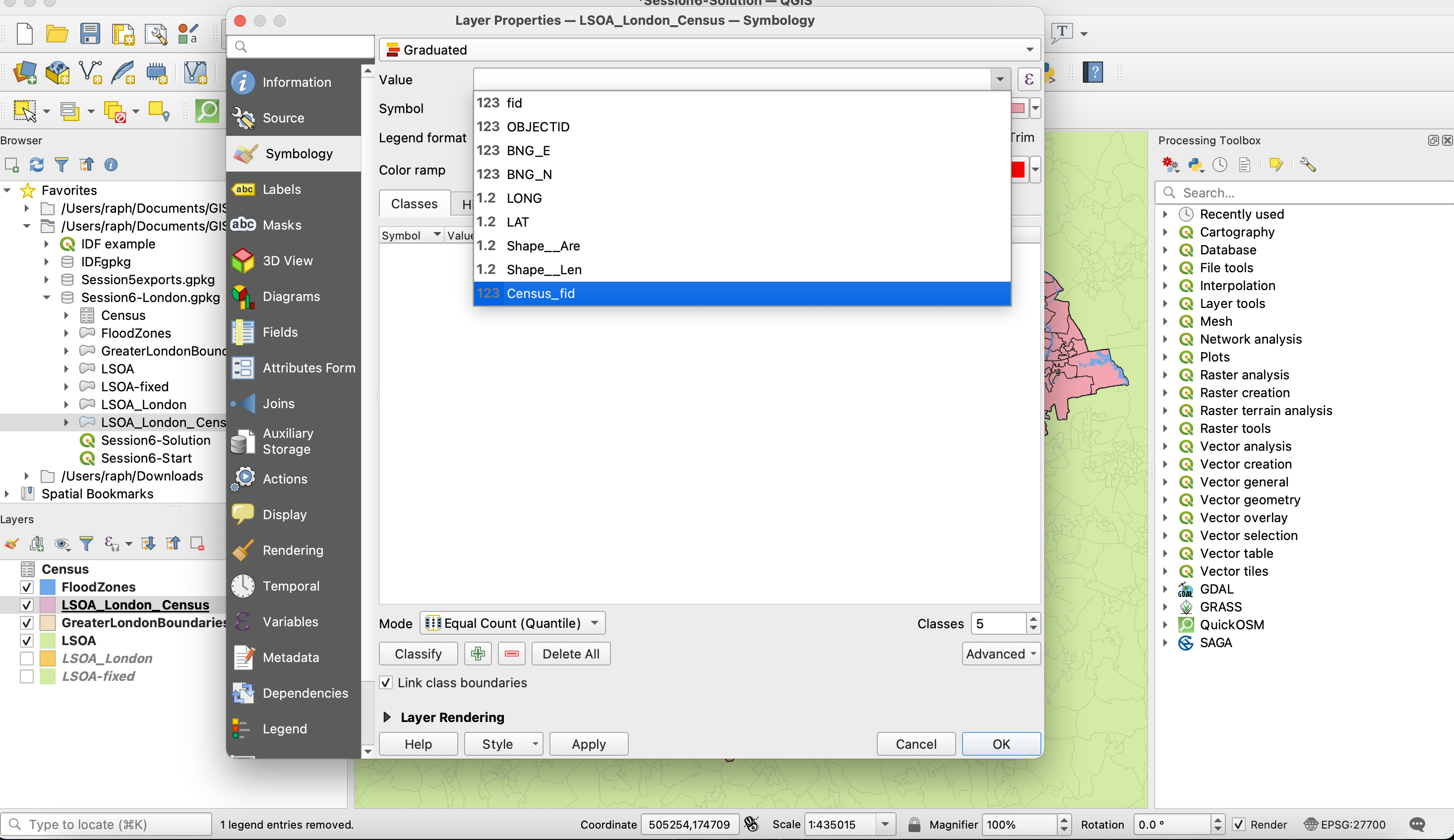
In your Symbology tab, you should find that your new PopDensity field is now available for Graduated symbology. Click Classify to bring up the values.
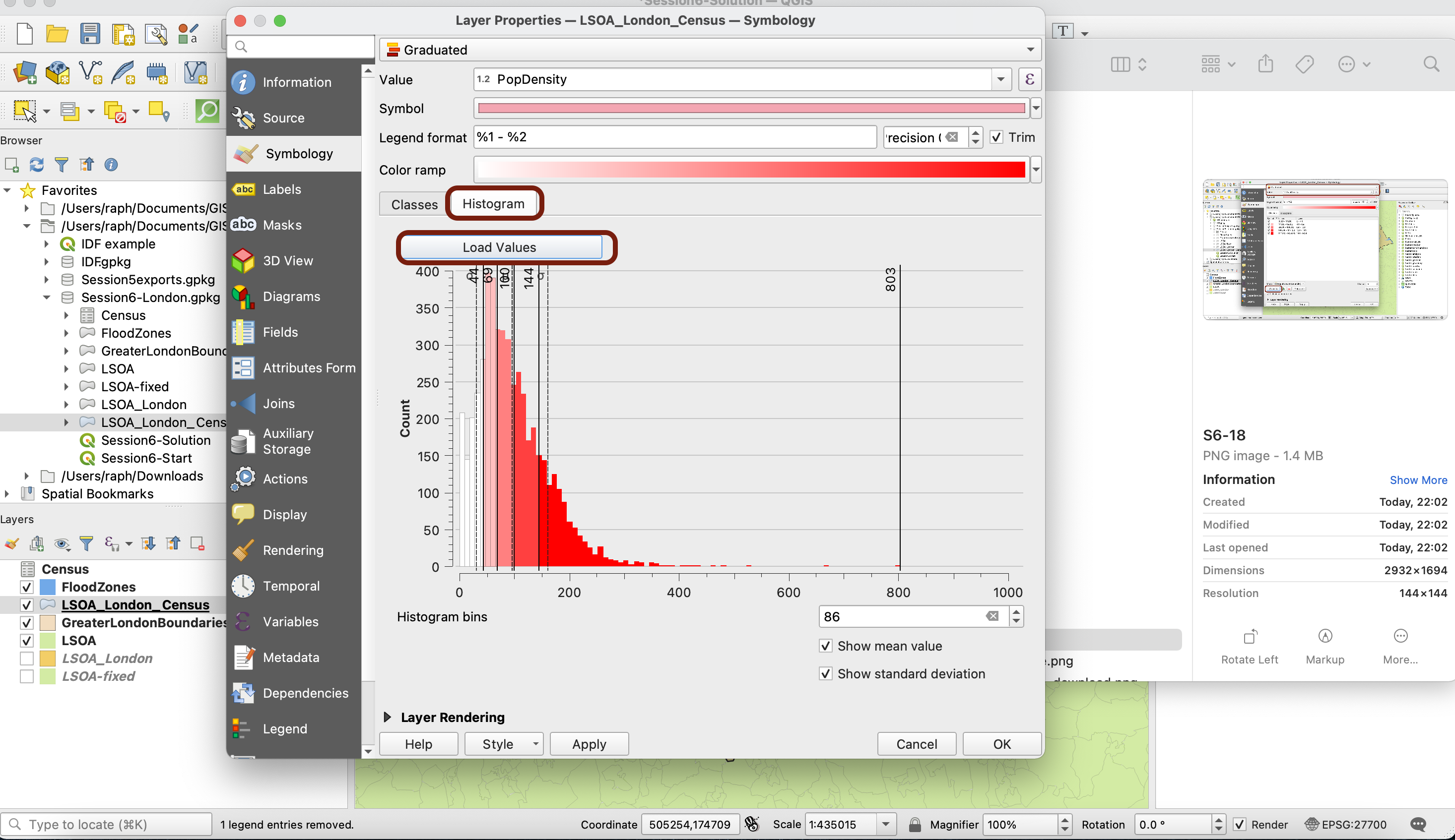
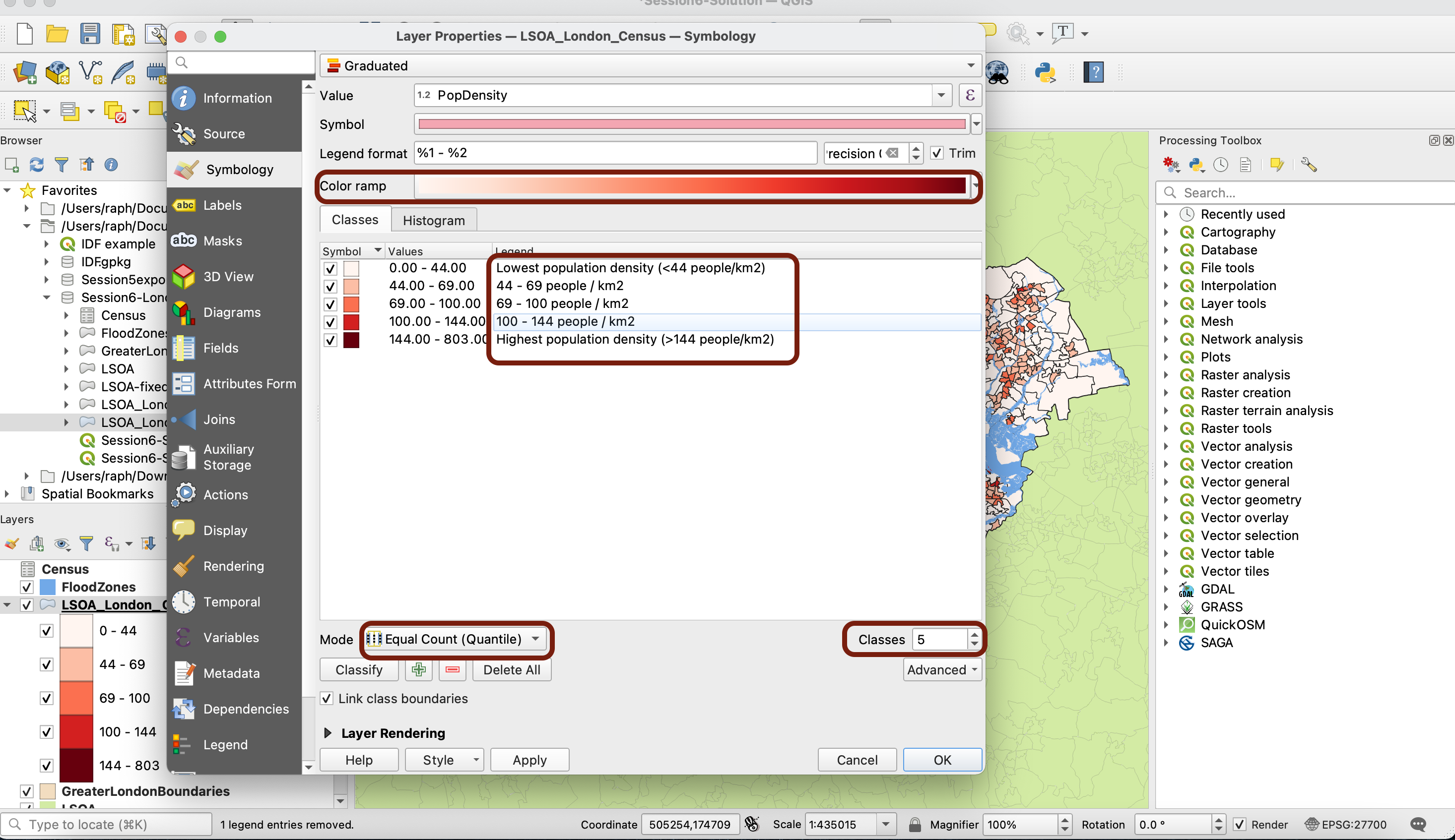
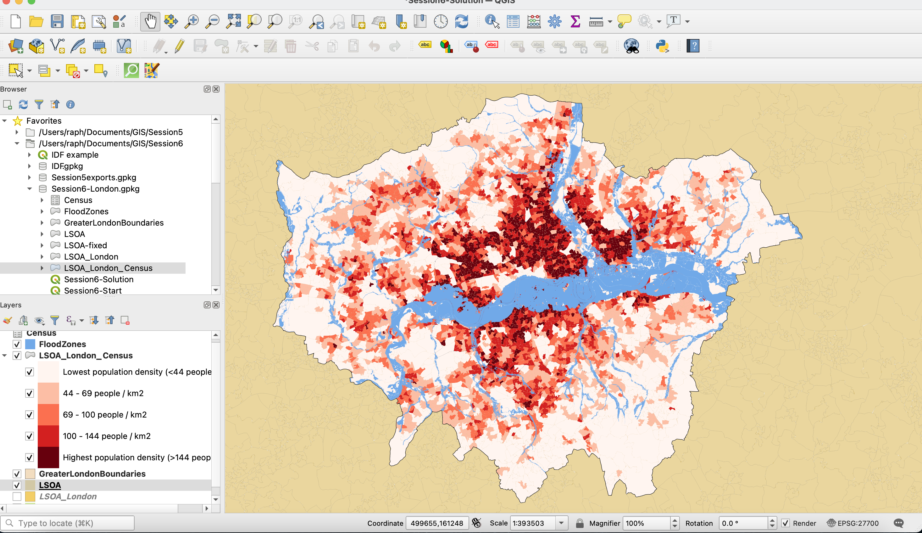
Click on the Histogram tab and Load values to see the distribution of your variables. As you can see, the distribution is not symmetrical and is right-skewed (the mean, mode and median are concentrated towards the left and the tail is to the right). In this case, it makes sense to use Equal count (quantile) as classification method because we want to emphasize the relative position between LSOAs. 5 classes is also a good number, and will allow us to visualise clearly the top 20% LSOAs with the highest population density, then the next 20%, and the next, all the way to the bottom 20% with lowest population density.
You can choose the Reds colour ramp for a nice range of reds, and you can manually edit the legend to reflect what the values mean.
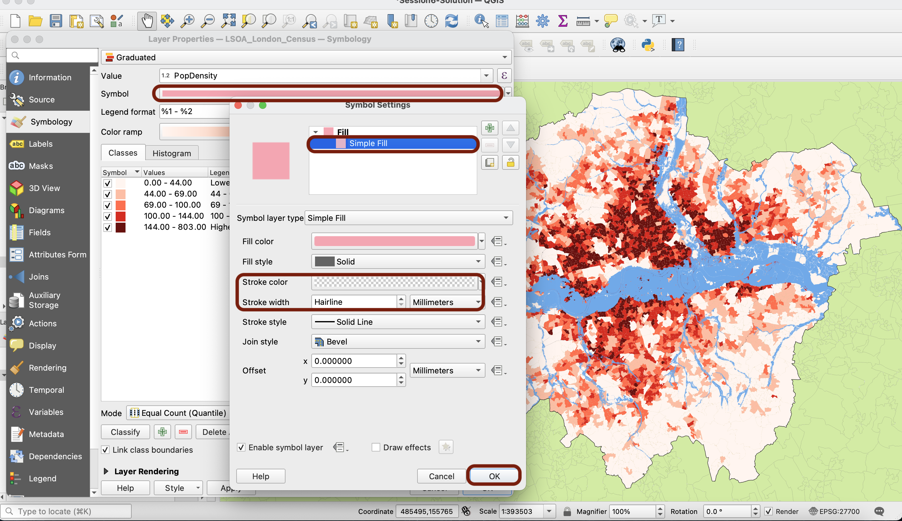
Now, two nice tips to improve your map symbology: click on your symbol to access customisations that will apply to all the colours in your colour ramp. First, click on Simple Fill and reduce the outline of your polygons to Hairline width and to a transparent colour.
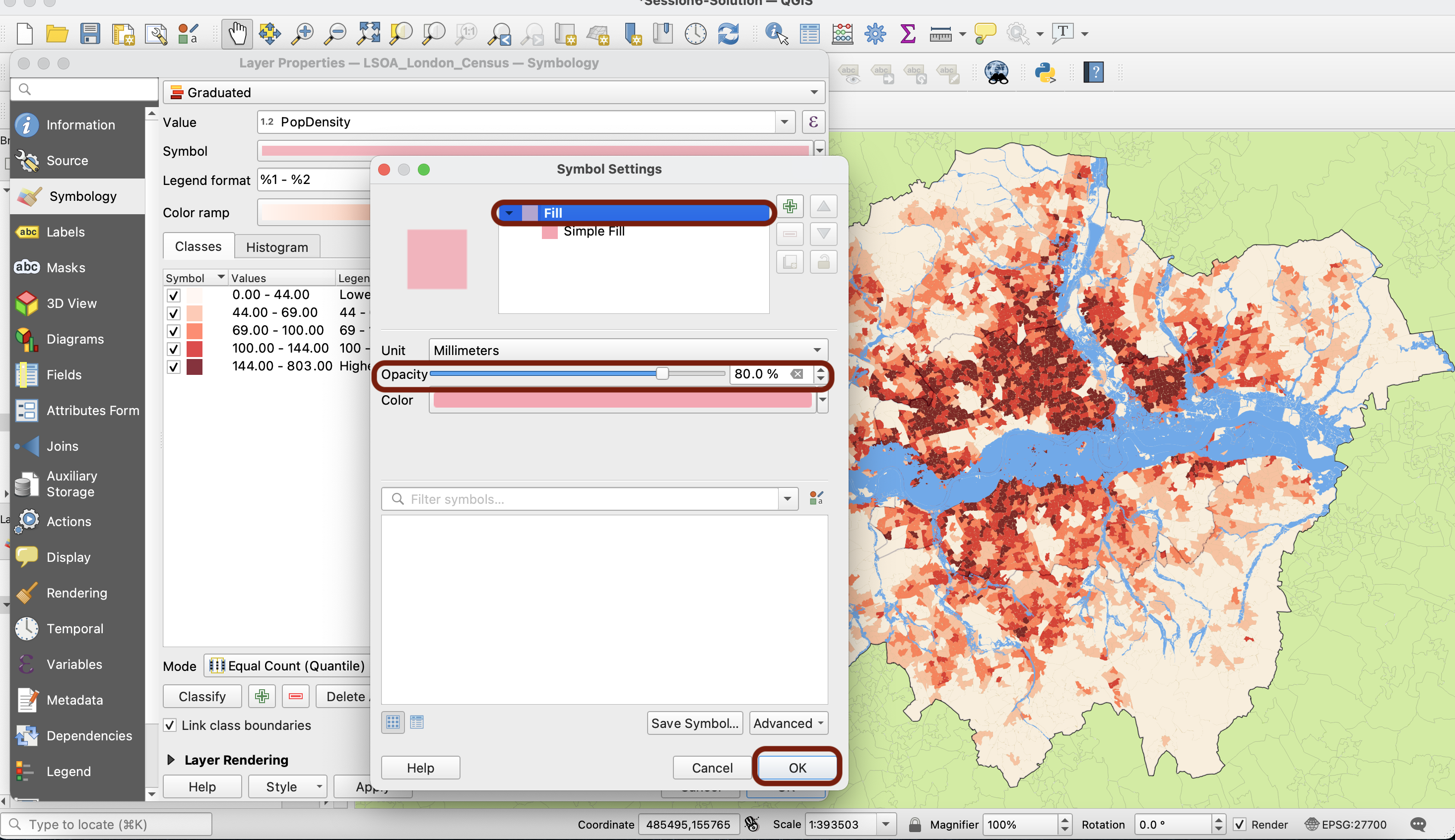
Next, click on Fill and reduce opacity to 80% to tone down slightly the colours.
Because we are using a red colour ramp, I’m also changing the UK LSOA layer to something else than green
V. Flood risk
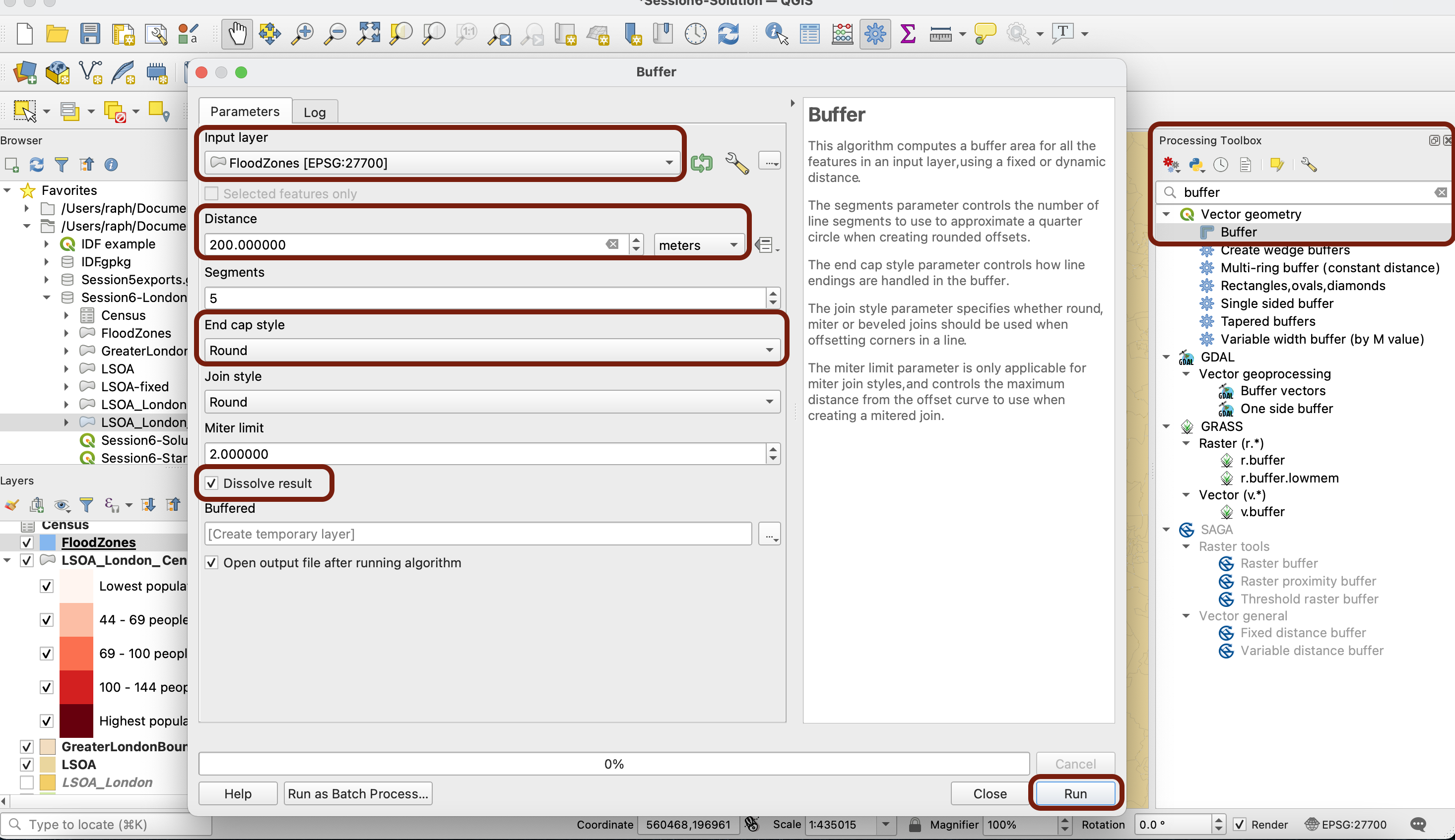
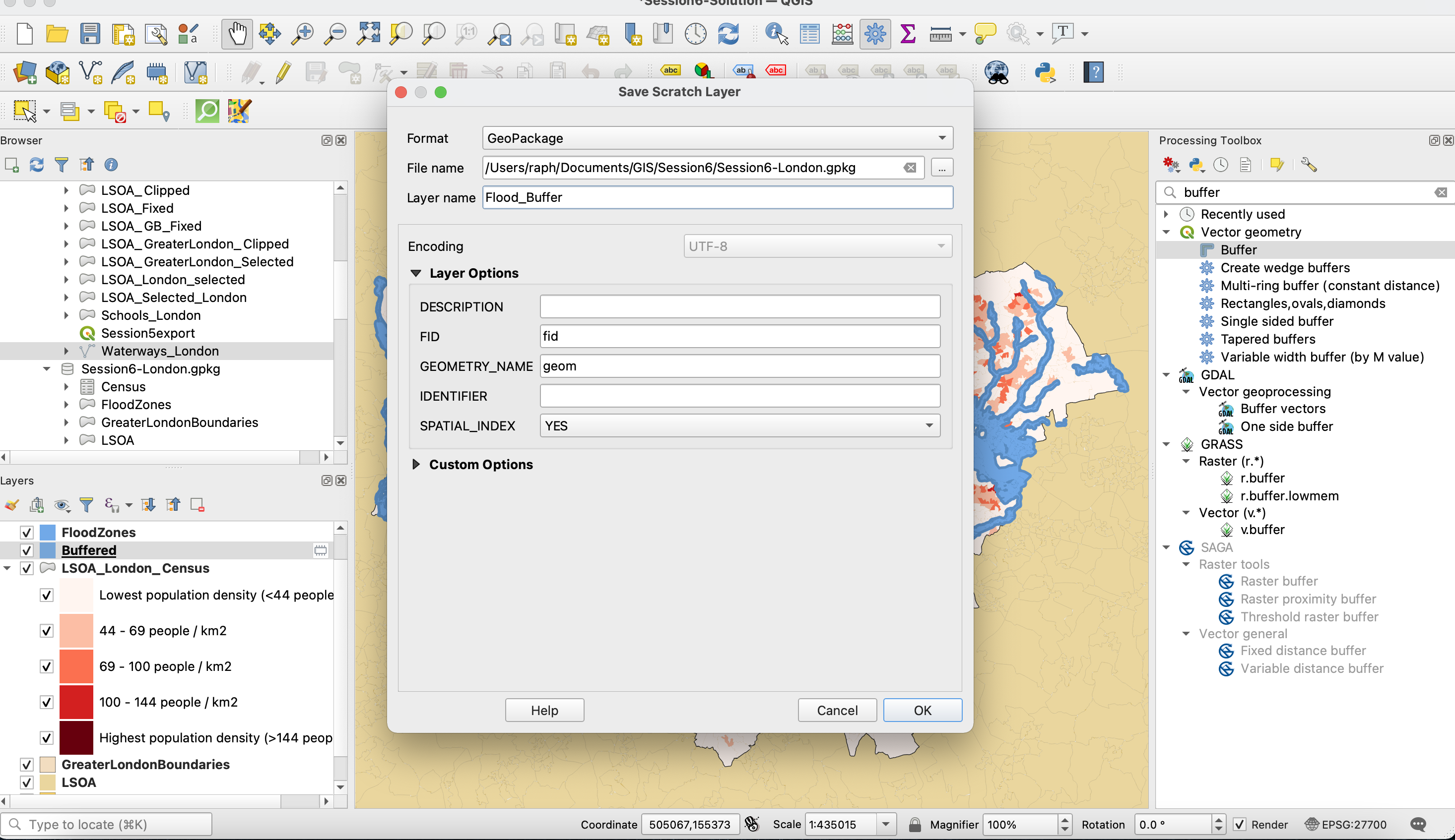
Finally, we want to find out which areas are exposed to flood risks. Say you want to be even more conservative than the risk models, and examine areas that are within 200m of a flood risk zone. In order to do that you can use the buffer geoprocessing tool.
Use your floodzone layer as input, define the distance and the unit (here 200m), and an end cap and join style (how your buffer ends an what the offset looks like). Tick “dissolve results” so that we end up with one large polygon rather than multiple overlapping polygons
Make sure to save that buffered layer!
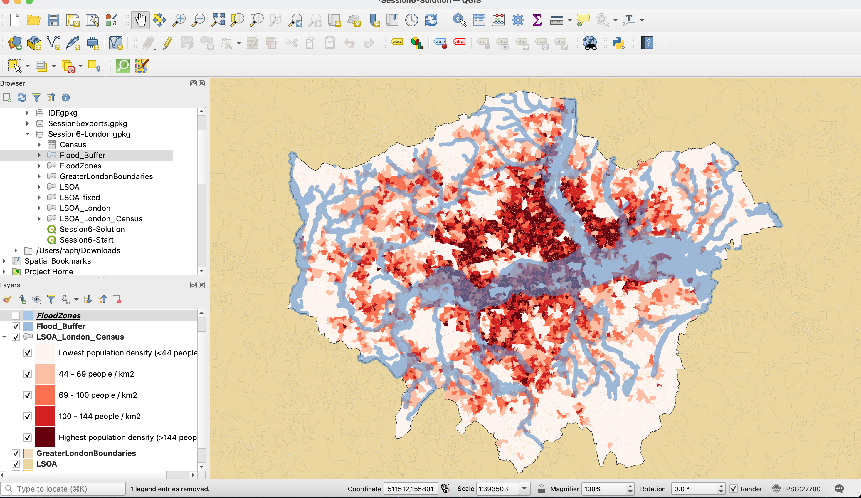
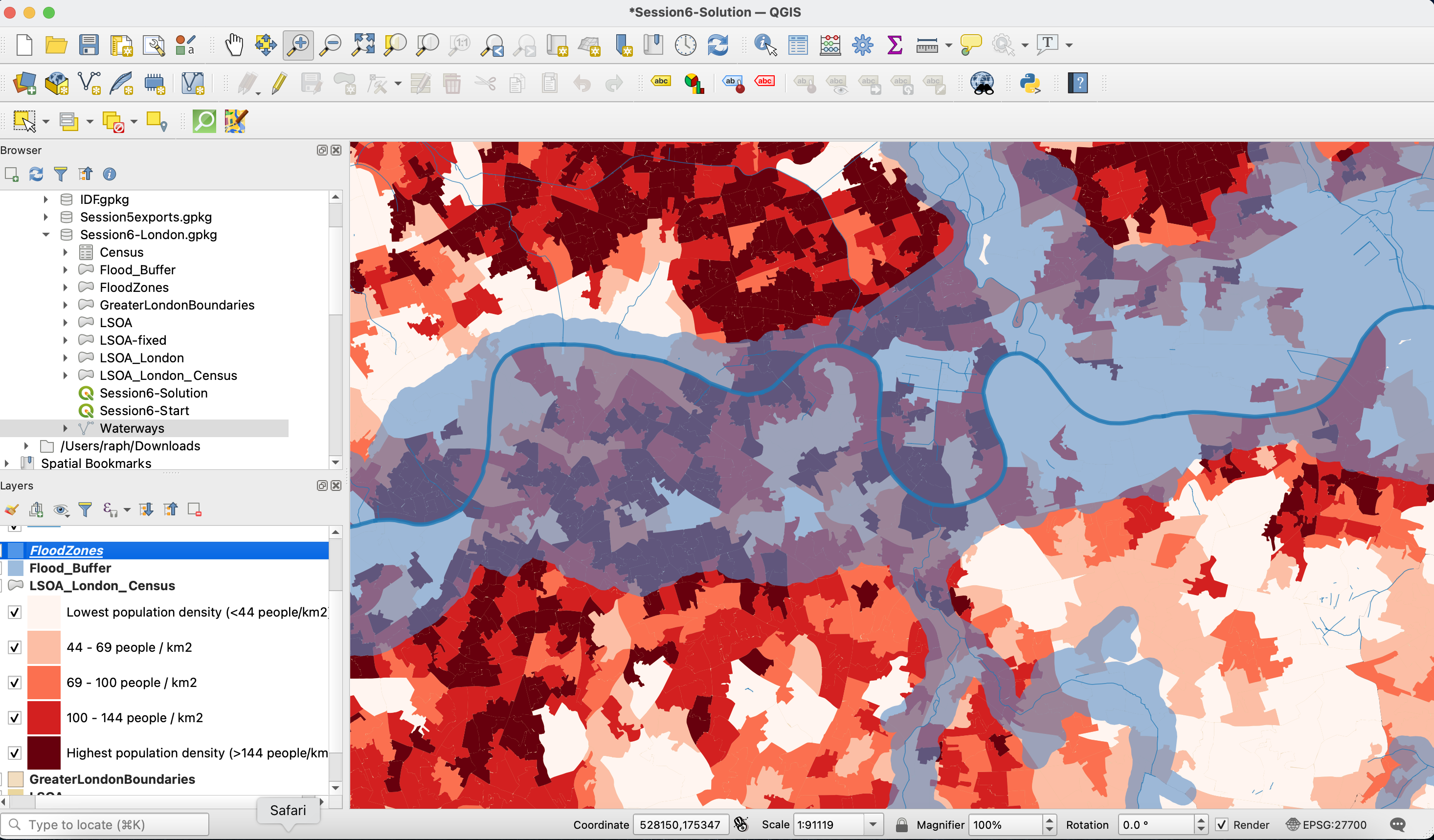
You can then play with your layer’s opacity to make sure the LSOA information is still accessible within those flood risk zones.
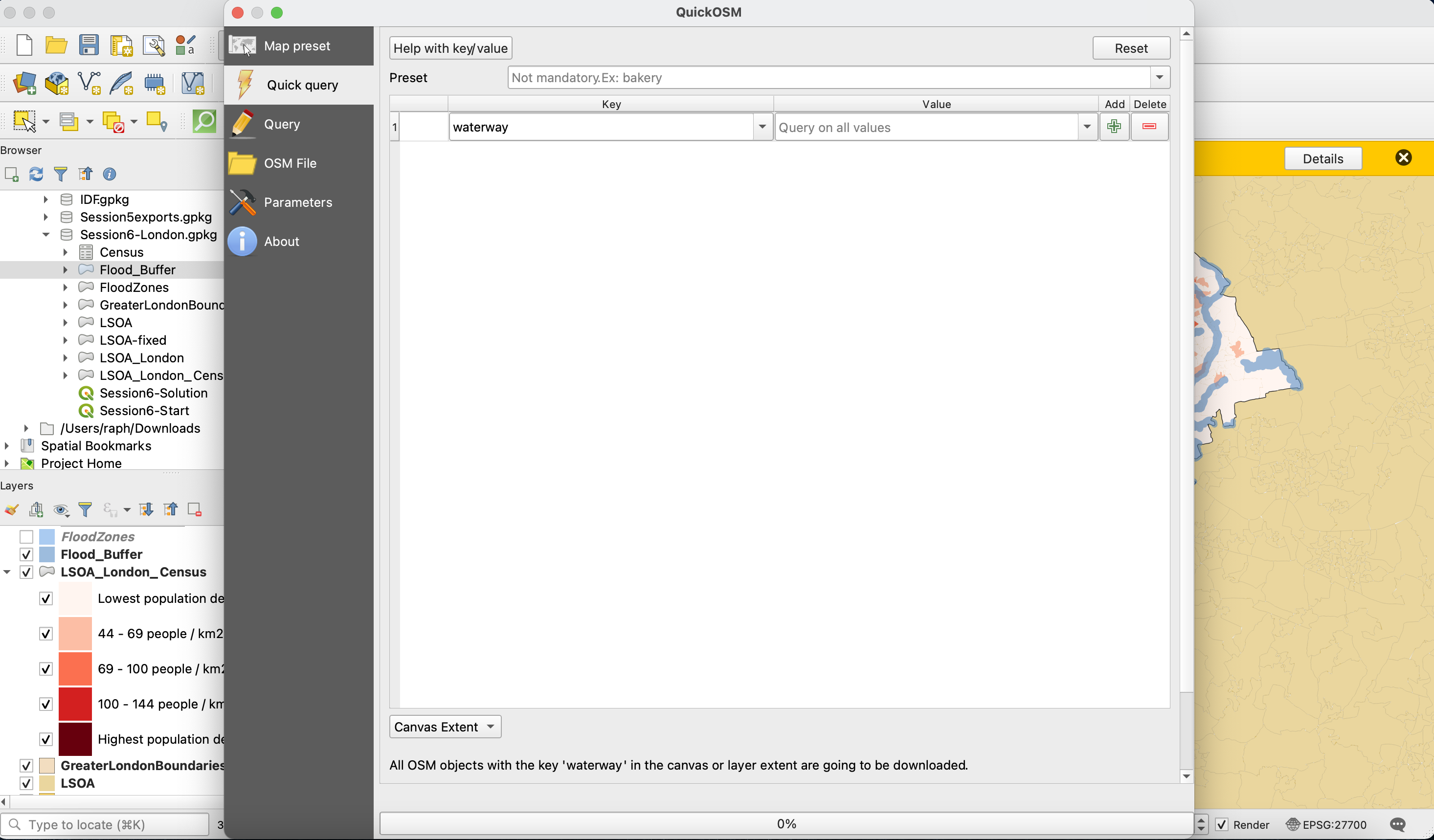
As a final step, you may want to bring in some data about the waterways. You can do so using QuickOSM; a copy of the query I ran is available in the geopackage as Waterways.
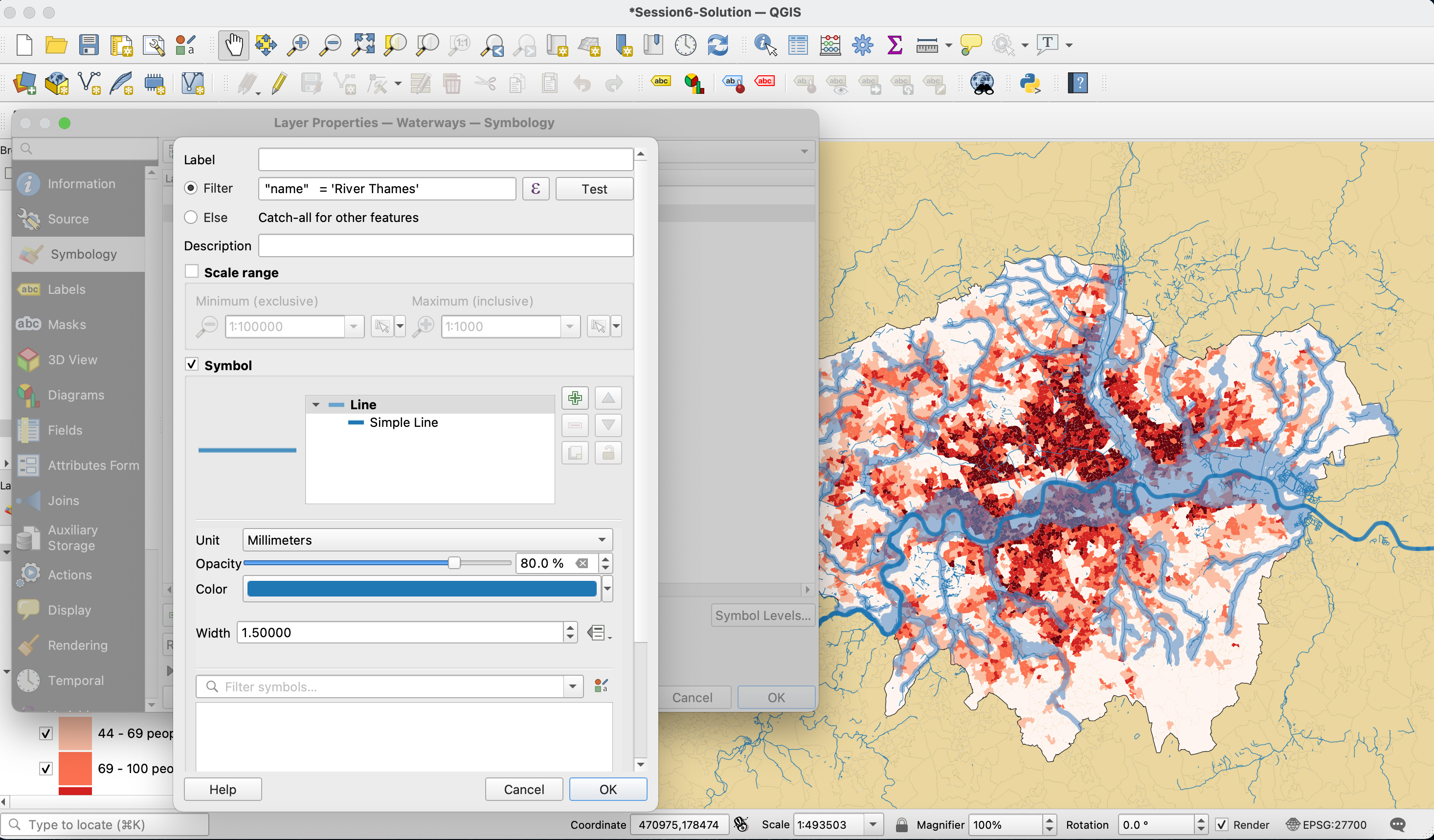
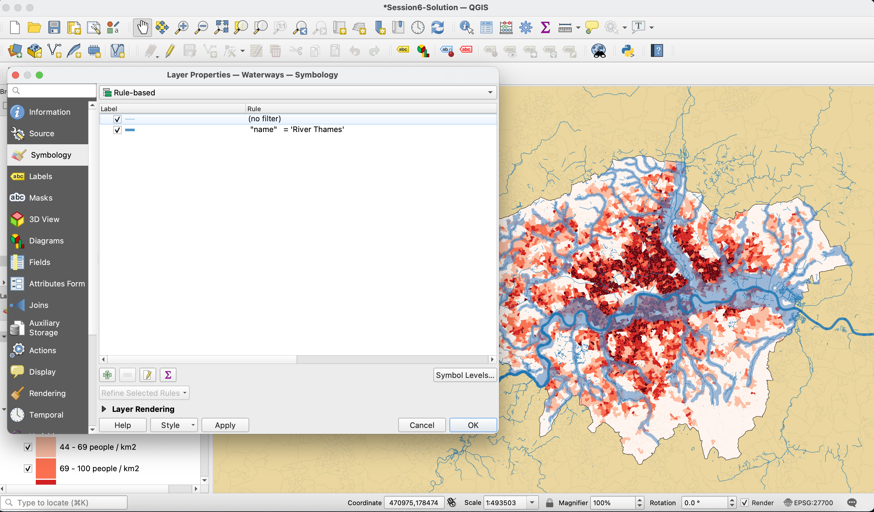
Because the Thames river is so much larger than other waterways in London, I’ll use a rule-based symbology to make the width larger (1.5) when "name" = 'River Thames', and thinner otherwise.
Your map is ready for you to explore! Use the Zoom to look into specific neighbourhoods and their exposure to flood risk. What new research questions do these observations raise? Which other census variable could provide useful insights into flood risk and population demographics?
Congratulations, you have now completed the Introduction to GIS course. Hopefully, this course and series of tutorials have picked your interest and you’re now ready to go further and start building more advanced analysis workflows. The Advanced GIS course will give you some new tools and methods to go further in your GIS practise - see you then!